Surfacing Point Sets with Fast Winding Numbers

Winding number of different regions inside and outside a mesh with self-intersecting and overlapping components.

In my previous tutorial on creating a 3D bitmap from a triangle mesh, I used the Mesh Winding Number to robustly voxelize meshes, even if they had holes or overlapping self-intersecting components. The Mesh Winding Number tells us “how many times” a point p is “inside” a triangle mesh. It is zero when p is outside the mesh, 1 if it is inside one component, two if it is inside twice, and so on, as illustrated in the image on the right. The Winding Number is an integer if the mesh is fully closed, and if there are holes, it does something reasonable, so that we can still pick an isovalue (say 0.5) and get a closed surface.

This is a very powerful technique but it is also very slow. To compute the Mesh Winding Number (MWN) for a given point p, it is necessary to evaluate a relatively expensive trigonometric function for each triangle of the mesh. So that’s an O(N) evaluation for each voxel of an O(M^3) voxel grid. Slow.

The original Winding Number paper by Jacobson et al had a neat trick to optimize this evaluation, which takes advantage of the fact that if you are outside of the bounding box of an “open” patch of triangles, the summed winding number for those triangles is the same as the sum over a triangle fan that “closes off” the open boundary (because these two numbers need to sum to 0). We can use this to more efficiently evaluate the winding number for all the triangles inside a bounding box when p is outside that box, and this can be applied hierarchically in a bounding-box tree. This optimization is implemented in DMeshAABBTree3.WindingNumber(). However, although this gives a huge speedup, it is not huge enough - it can still take minutes to voxelize a mesh on a moderately-sized grid.

At SIGGRAPH 2018, I had the pleasure to co-author a paper titled Fast Winding Numbers for Soups and Clouds with Gavin Barill, Alec Jacobson, and David Levin, all from the University of Toronto’s DGP Lab, and Neil Dickson of SideFX. As you might have gathered from the title, this paper presents a fast approximation to the Mesh Winding Number, which also can be applied directly to surface point sets. If you are interested in C++ implementations, you can find them on the paper’s Project Page. In this tutorial I will describe (roughly) how the Fast Winding Number (FWN) works and how to use the C# implementation in my geometry3Sharp library, which you can find on Nuget or Github.

[Update 09-26-18] Twitter user @JSDBroughton pointed out that in the above discussion I claim that the Winding Number is an integer on closed meshes. This is true in the analytic-math sense, however when implemented in floating point, round-off error means we never get exactly 0 or 1. And, the approximation we will use below will introduce additional error. So, if you want an integer, use Math.Round(), or if you want an is-this-point-inside test, use Math.Abs(winding_number) > 0.5.

Fast Winding Number Approximation

solid_angle.png

The key idea behind the Fast Winding Number is that if you are “far away” from a set of triangles, the sum of their individual contributions to the overall mesh winding number can be well-approximated by a single function, ie instead of evaluating N things, you evaluate 1. In the Mesh Winding Number, the contribution of each triangle is it’s solid angle measured relative to evaluation point p. The figure on the right illustrates what the solid angle is - the area of the projection of the 3D triangle onto a sphere around p, which is called a spherical triangle.

When p is relatively close to the triangle, like in the figure, then any changes to the 3D triangle will have a big effect on this projected spherical triangle. However, if p is “far away” from the triangle, then its projection will be small and changes to the triangle vertices would hardly change the projected area at all. So, when the triangle is far away, we might be able to do a reasonable job of numerically approximating its contribution by replacing it with a small disc. In this case, instead of a 3D triangle we would have a point, a normal, and an area.

Of course, replacing an O(N) evaluation of triangles with an O(N) evaluation of discs would not be a big win. But, once we have this simplified form, then through some mathematical trickery, the spherical angle equation can be formulated as a mathematical object called a dipole. And the sum of a bunch of dipoles can be approximated by a single dipole, if you are far enough away. The figure on the right, taken from the paper, shows a 2D example, where the sum of 20 dipoles is approximated by a single stronger dipole. Even at relatively small distances from the cluster of dipoles, the scalar field of the sum is hardly affected by replacing the simplification.

This is how we get an order-of-magnitude speedup in the Winding Number evaluation. First we compute an axis-aligned bounding volume hierarchy for the mesh. Then at each internal node of the tree, we find the coefficients of a single dipole that approximate the winding number contributions for each triangle below that node. When we are evaluating the Winding Number later, if the evaluation point p is far enough away from this node’s bounding box, we can use the single-dipole approximation, otherwise we recursively descend into the node. Ultimately, only the triangles very near to p will actually have their analytic solid angles evaluated. The speedups are on the order of 10-100x, increasing as the mesh gets larger. It is…super awesome.

Also, since the dipole is a function at a point, we can apply this same machinery to a set of points that are not connected into triangles. We will still need a normal and an “area estimate” for each point (more on that below). But the result will the a 3D scalar field that has all the same properties as the Mesh Winding Number.

Mesh Fast Winding Number

There really isn’t much to say about using the Mesh Fast Winding Number. Instead of calling DMeshAABBTree3.WindingNumber(), call FastWindingNumber(). They behave exactly same way, except one is much faster, at the cost of a small amount of approximation error. Note that the internal data structures necessary to do the fast evaluation (ie the hierarchy of dipole approximation coefficents) are only computed on the first call (for both functions). So if you are planning to do multi-threaded evaluation for many points, you need to call it once before you start:

DMeshAABBTree3 bvtree = new DMeshAABBTree3(mesh, true);
bvtree.FastWindingNumber(Vector3d.Zero);   // build approximation
gParallel.ForEach(list_of_points, (p) => {
    double winding_num = bvtree.FastWindingNumber(p);
});

There are a few small knobs you can tweak. Although the paper provides formulas for up to a 3rd order approximation, the current g3Sharp implementation is only second-order (we don’t have a third-order tensor yet). You can configure the order you want using the DMeshAABBTree3.FWNApproxOrder parameter. First order is faster but less accurate. Similarly, the parameter DMeshAABBTree3.FWNBeta controls what “far away” means in the evaluation. This is set at 2.0, as in the paper. If you make this smaller, the evaluation will be faster but the numerical error will be higher (I have never had any need to change this value).

Point Fast Winding Number

geometry3Sharp also has an implementation of the Fast Winding Number for point sets. This involves several interfaces and classes I haven’t covered in a previous tutorial. The main class we will need to use is PointAABBTree3, which works just like the Mesh variant. However, instead of a DMesh3, it takes an implementation of the IPointSet interface. This interface just provides a list of indexed vertices, as well as optional normals and colors. In fact DMesh3 implements IPointSet, and works fine with “only” vertices. So we can use a DMesh3 to store a point set and build a PointAABTree3, or you can provide your own IPointSet implementation.

To test the Point Fast Winding Number implementation, we will use a mesh of a sphere. Here is a bit of sample code that sets things up:

Sphere3Generator_NormalizedCube gen = new Sphere3Generator_NormalizedCube() { EdgeVertices = 20 };
DMesh3 mesh = gen.Generate().MakeDMesh();
MeshNormals.QuickCompute(mesh);
PointAABBTree3 pointBVTree = new PointAABBTree3(mesh, true);

Now, I mentioned above that each point needs a normal and an area. We computed the normals above. But the per-point areas have a big effect on the resulting iso-surface, and there is no standard “right way” to compute this. In this case, since we know the point sampling of the sphere is approximately regular, we will assume the “area” of each point should be a disc around it, with radius equal to half the average point-spacing. Here is a way to calculate this:

double mine, maxe, avge;
MeshQueries.EdgeLengthStats(mesh, out mine, out maxe, out avge);
Circle2d circ = new Circle2d(Vector2d.Zero, avge * 0.5);
double vtxArea = circ.Area;

The way we tell PointAABBTree3 about the per-vertex area estimates is to provide an implementation of the lambda function FWNAreaEstimateF:

pointBVTree.FWNAreaEstimateF = (vid) => {
    return vtxArea;
};

Now we can call pointBVTree.FastWindingNumber(), just like the mesh version. Now, say you would like to generate a mesh surface for this winding number field. We can easily do this using the MarchingCubes class. We just need to provide an ImplicitFunction3d implementation. The following will suffice:

class PWNImplicit : BoundedImplicitFunction3d {
    public PointAABBTree3 Spatial;
    public AxisAlignedBox3d Bounds() { return Spatial.Bounds; }
    public double Value(ref Vector3d pt) {
        return -(Spatial.FastWindingNumber(pt) - 0.5);
    }
}

Basically all we are doing here is shifting the value so that when the winding number is 0, ie “outside”, the scalar field value is -0.5, while it is 0.5 on the “inside”, and 0 at our “winding isosurface”, where the winding number is 0.5. We have to then negate these values because all our implicit surface machinery assumes that negative == inside.

Finally, this bit of code will do the surfacing, like in our previous implicit surface tutorials. Note that here we are using a cube resolution of 128, you can reduce this for quicker, lower-resolution results. It is also quite important to use the Bisection root-finding mode. The default is to use linear interpolation, but because of the “shape” of the winding number field, this will not work (as is described in the paper).

MarchingCubes mc = new MarchingCubes();
mc.Implicit = new PWNImplicit() { Spatial = pointSpatial };
mc.IsoValue = 0.0;
mc.CubeSize = pointSpatial.Bounds.MaxDim / 128;
mc.Bounds = pointSpatial.Bounds.Expanded(mc.CubeSize * 3);
mc.RootMode = MarchingCubes.RootfindingModes.Bisection;
mc.Generate();
DMesh3 resultMesh = mc.Mesh;

The result of running this code is, as expected, a mesh of a sphere. Not particularly exciting. But the point is, the input data was in fact just a set of points, normals, and areas, and through the magic of the Point Fast Winding Number, we turned that data into a 3D isosurface.

Area Estimates and Scan Surface Reconstruction

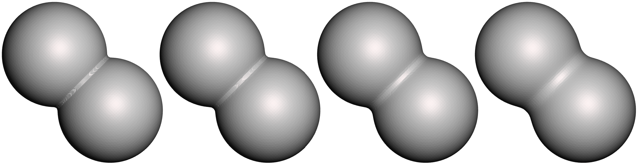
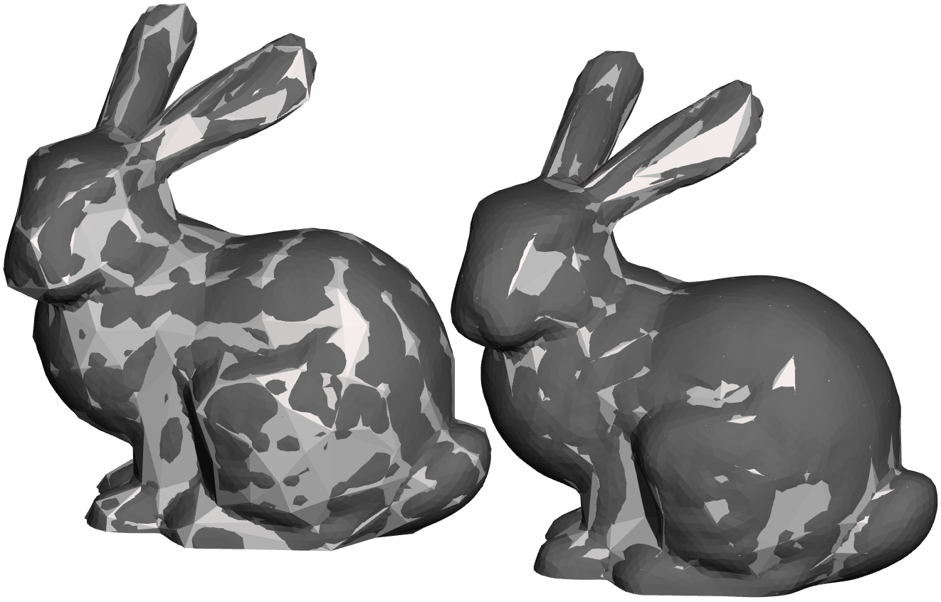
In the example above, we were cheating because we knew the point cloud came from a sphere, and specifically from a quite regular mesh of the sphere. This made it easy to get a sensible per-vertex area estimate. What if our estimate was not so good? An interesting experiment is just to scale our fixed per-vertex area. In the example below, we have the “correct” result on the left, and then the result with the area scaled by 2x, 4x, and 0.5x. The effects are neat, but also…not ideal for surface reconstruction.

Unfortunately there is no “right” way to assign an area to each point in a point cloud (in fact there is no “right” way to assign normals, either!). The Fast Winding Number paper describes a method based on using Delaunay Triangulations in local 2D planar projections around each point. This is a great way to do it, but it also involves several complicated steps, and can take quite a bit of time for a large point set. So, we’ll try something simpler below.

But first, we need a point set. For this test I will use a “real” point set, rather than a nice “synthetic” one that is sampled from a known triangle mesh. I am going to use the Chinese Dragon sample scan from the AIM@SHAPE 3D model repository. Actually I just used the “upper” scan, which contains 1,766,811 points, in XYZ format, which is a simple list of point positions and normals. You can directly open and view XYZ point cloud files Meshlab, a few screenshots are shown to the right. As you can see, the scan points are spaced very irregularly, and there are huge regions with no data at all! So, we cannot expect a perfect reconstruction. But if we could get a watertight mesh, then we can take that mesh downstream to tools where we could, for example, 3D sculpt the mesh to fix the regions where data was missing, take measurements for digital heritage applications, or just 3D print it.

Since the scanner provided (approximate) surface normals, the main thing we need to do is estimate an area for each point. This area clearly needs to vary per-point. We’ll try something just slightly more complicated than we did on the sphere - we’ll find the nearest-neighbour to each point, and use the distance to that point as the radius of a disc. The disc area will then be the point radius. Here’s the code:

DMesh3 pointSet = (load XYZ file here...)

// estimate point area based on nearest-neighbour distance
double[] areas = new double[pointSet.MaxVertexID];
foreach (int vid in pointSet.VertexIndices()) {
    bvtree.PointFilterF = (i) => { return i != vid; };   // otherwise vid is nearest to vid!
    int near_vid = bvtree.FindNearestPoint(pointSet.GetVertex(vid));
    double dist = pointSet.GetVertex(vid).Distance(pointSet.GetVertex(near_vid));
    areas[vid] = Circle2d.RadiusArea(dist);
}    
bvtree.FWNAreaEstimateF = (vid) => {
    return areas[vid];
};

Note that this is not the most efficient way to compute nearest-neighbours. It’s just convenient. Now we can run the MarchingCubes surfacing of the Point-Set Winding Number Field defined with these areas. The result is surprisingly good (I was, in fact, literally surprised by how well this worked - the first time, no less!). The images below-far-left and below-far-right show the raw Marching Cubes output mesh, at “256” resolution. There is some surface noise, but a Remeshing pass, as described in a previous tutorial, does a reasonable job of cleaning that up (middle-left and middle-right images). The only immediately-obvious artifact of the dirty hack we used to estimate surface areas seems to be that in a few very sparsely sampled areas (like the rear left toe) the surface was lost.

In areas where there were no surface points, the winding field has produced a reasonable fill surface. I can’t quite say “smooth” because one artifact of the Fast Winding Number approximation is that in the “far field”, ringing artifacts can be visible. This is an artifact of using a hierarchical evaluation of a functional approximation. At each point in space we have to make a decision about whether to use a finer approximation or not, and this decision varies over space. (One potential fix here would be to smoothly transition or“blend” between approximations at different levels, instead of picking one or the other - something for a reader to implement?)

Summary

Traditionally, determining point containment for an arbitrary 3D mesh has been problematic to use in many applications because there wasn’t a great way to compute it. Raycast parity-counting is not efficient and can go horribly wrong if the mesh has imperfections, and voxelizing is memory-intensive and similarly fails on many real-world meshes. The Mesh Winding Number provides a much better solution, and the Fast Winding Number approximation makes it practical to use, even on huge meshes at runtime.

For example I have encountered many situations in building VR user interfaces where I want to be able to check if a point (eg on a spatial controller) is inside a 3D UI element (eg for selection). In most cases I would need to approximate the UI element with simpler geometric bounding-objects that support analytic containment tests. With the Fast Winding Number, we can now do these tests directly on the UI element.

Remeshing and Mesh Constraints

tmp.png

Recently geometry3Sharp user samyuchao asked a question about a topic I've been meaning to write about for nearly a year. The question was, for the mesh on the right, how to re-triangulate it so that the triangles are uniform but the boundary shape is preserved. This can easily be done with the geometry3Sharp Remesher class, with just a few lines of code. 

Before we begin, I'll just mention that although this tutorial is about using the Remesher directly from C#, you can do the same experiments using the Remesh Tool in Gradientspace's Cotangent app, because it uses the same Remesher class internally. You can get Cotangent here

The Remesher class works much like the Reducer class I covered in a previous tutorial. In fact they both inherit from MeshRefinerBase which provides common functionality based on the MeshConstraints we will use below. Here is the minimal code to run a remesh:

DMesh3 mesh = load_my_mesh_somehow();
Remesher r = new Remesher(mesh);
r.PreventNormalFlips = true;
r.SetTargetEdgeLength(0.5);
for ( int k = 0; k < 20; ++k )
    r.BasicRemeshPass();

If we run this code on our standard bunny mesh, we get the result to the right. There are a few things to explain here. First of all, the goal of Remesher is to create a uniform or isotropic mesh. So, we give it an edge-length goal, and it tries to convert the input mesh into one where all the edges have that length. In fact, as I will explain below we need to give it both a minimum and maximum edge length, because we can't achieve exactly a specific length. The function SetTargetEdgeLength() sets suitable min/max lengths based on the given goal length, but you can also directly set .MinEdgeLength and .MaxEdgeLength. Note that this is an absolute length, so it needs to be defined to a value that makes sense for your input mesh (in this case our standard bunny has an average edge length of 1.0, which keeps things simple). See below for tips about calculating a relative edge length.

Next we do 20 iterations of BasicRemeshPass(). I will explain what this does below, but the main thing to understand is that Remesher does iterative mesh refinement or mesh optimization. That means we take "steps" towards our goal, in the form of passes. More passes means better results, but also more compute time. 

You may also have noticed that in the above-right example, the surface has been smoothed out. This is because our mesh refinement is combined with mesh smoothing. This smoothing is necessary to achieve the reguarly-shaped triangles, but as an artifact the surface shrinks. The .SmoothSpeedT property controls how quickly the smoothing happens. More passes means more smoothing, which can mean that if you want to get a very regular triangulation, your object will shrink a lot. Maybe this is what you want, though! In the grid of images to the right, SmoothSpeedT is set to 0.1, 0.25, and 1.0 in the 3 rows, and the columns are after 20, 40, and 60 iterations. In this case I used a target edge length of 1 (Click on this image to make it bigger).

Projection Targets

Most of the time where we would like to use remeshing, we don't want to smooth out the shape so drastically. We just want to improve the mesh quality and/or modify triangle density. To preserve the shape we need to reproject the evolving mesh onto the input surface. We can do this with a slight modification to the Remesher setup:

r.SetTargetEdgeLength(0.75);
r.SmoothSpeedT = 0.5;
r.SetProjectionTarget(MeshProjectionTarget.Auto(mesh));
(...remesh passes...)

MeshProjectionTarget.Auto() is a utility function that copies the input mesh and creates a DMeshAABBTree3 bounding-box hierarchy (which I covered in a previous tutorial). A copy is required here because we are going to modify the mesh in Remesher, if you already have a copy lying around, MeshProjectionTarget has other constructors that can re-use it. Here's the result of running this code for 20 iterations with SmoothSpeedT = 0.1 and 0.5:

In this case we can see that SmoothSpeedT has a different effect - the triangulation is much less regular in the middle image. This is what happens when you increase triangle density but smooth slowly - the triangles do not have "time" to redistribute themselves evenly. You might be thinking, well why don't I just always crank it up to 11 (or 1 in this case)? Well, here is another example:


In the leftmost image we set the target length to 1.5 (so, larger triangles than our initial mesh) and SmoothSpeedT to 1. The thin areas of the ears have eroded away. What happens in this case is that as we smooth and reproject the vertices, they tend to clip off bits of the thin extremities each pass. Because we are taking large smoothing steps, this happens very quickly. If we take smaller steps (SmoothSpeedT=0.1 in the middle), this happens more slowly. On the right, we have set a configuration flag Remesher.ProjectionMode = Remesher.TargetProjectionMode.Inline. Normally, we compute a smoothing pass, and then a projection pass. When we set the projection mode to Inline, we immediately compute the projected position of each vertex. This is less efficient but can reduce erosion of the thin features.

However, ultimately, Remesher is not a great way to drastically reduce the resolution of a mesh, because of the smoothing process (unless you have constraints that will preserve features, more on this below). Reducer is a much better choice if you want to really minimize triangle counts.

Note also that you can actually use any surface as the projection target, or even use more complicated programmatic projection targets. You can get many interesting effects this way. For example, in the screenshot on the right I am using Cotangent's Map To Target Tool in Bounded mode, to remesh the green bunny using the purple box as the target. This mode uses a custom projection target that smoothly blends between projecting onto the box, and projecting onto the bunny, based on a distance falloff. This produces a kind of surface-blending operation that would be quite difficult to achieve any other way. 

How does it work?

edge_ops.png

As I mentioned above, the Remesher class uses an implementation of iterative mesh refinement. What "iterative" means here is that we make passes over the mesh and in each pass we make improvements that get us closer to our goal (in this case a uniform mesh). Further down the page there are a few videos that show the evolving state of a mesh after each pass.

Inside each pass, we iterate over the edges of the mesh and apply one three operations - FlipSplit, or Collapse. The diagram to the right shows what happens in each of these operations. A Flip (sometimes called an edge "rotation") replaces two triangles with two new  triangles. A Split replaces two triangles with four new ones, by adding a vertex. By default this vertex is placed on the original edge, so a Split is the one operator we can do that is guaranteed to not change the mesh shape. Finally Collapse is used to remove an edge. This is is the most drastic change (and hardest to implement correctly!) because the one-rings of all four vertices of the initial triangle-pair are affected.

Mesh boundary edges can be can Split and Collapsed, but not Flipped. The DMesh3 implementations of these operations - SplitEdge()CollapseEdge(), and FlipEdge(), will also not allow changes that would result in non-manifold mesh topology, such as an edge with more than two connected triangles. 

smooth_ops.png

As I mentioned above, These edge operators are combined with mesh smoothing. The Remesher uses standard Laplacian smoothing with uniform weights, which maximizes inner fairness, ie triangle regularity. Unfortunately it also means the shape changes the most quickly. If you have a case where the triangle shapes need to be preserved (for example if the mesh has UVs), you can try changing the .SmoothType property - Cotangent and Mean Value weights are also implemented. 

Since the edge operators and smoothing are all applied locally, the order of operations matters - we call this the "remeshing policy". A standard approach is to do passes of each operator. Remesher does not do this as it results in much wasted work on large meshes, particularly as the mesh converges (just checking if we need to flip any edges on a million triangles is quite expensive). The policy in Remesher is as follows:

foreach ( edge in current_mesh ) {
    if ( edge too short ) collapse_edge();
    elif ( edge needs flip ) flip_edge();
    elif ( edge too long ) split_edge();
}
smooth_all_vertices();
reproject_all_vertices();

The outer steps are defined in BasicRemeshPass() and ProcessEdge(). The code for each of the inner steps is relatively clearly demarcated, and should be relatively easy to cut-and-paste if you wanted to re-organize this into separate flip/split/collapse passes. If you are interested in the academic research behind this, Remesher is in large part an implementation of the techniques described in A Remeshing Approach to Multiresolution Modeling (Botsch and Kobbelt, SGP 2004).

Boundary Constraints

So far we've been dealing with close meshes, but the original question was about a mesh with an open boundary. What happens if we run the code above on a mesh-with-boundary? Nothing good! As the boundary vertices are smoothed, some of the edges get shorter and are collapsed, which basically means that the open boundary erodes away. 

To fix this we will need to configure Remesher.Constraints, which is an instance of the MeshConstraints class. This class allows you to set constraints on the mesh edges and vertices, based on their IDs. Edges can be restricted so that they can't be flipped, collapsed, split, or any combination of these. Edges can also be associated with a particular IProjectionTarget. Similarly vertices can be constrained to be fixed in place, or allowed to slide along an IProjectionTarget.

To constrain the open boundaries of a mesh, we can use the helper class MeshConstraintsUtil as follows:

Remesher r = new Remesher(mesh)
MeshConstraintUtil.FixAllBoundaryEdges(r);

This will create a MeshConstraints instance and populate it with the boundary edge and vertex constraints. It's actually only a few lines of code, so if you want to experiment with setting up your own constraints, this is a good starting point. For these examples I'll use a flat mesh with boundary as it's easier to see what is happening. On the left we have the input mesh, and in the middle is the result using the above constraints. As you can see, the boundary is preserved. In fact it has been exactly preserved - exact same vertices in the same locations. This can be useful (eg if you want to remesh in parts and stitch back together later) but it does mean that there will be ugly triangles around the border, just like in samyuchao's example. So how do we get to the example on the right?

Instead of FixAllBoundaryEdges(), we can use the following:

MeshConstraintUtil.PreserveBoundaryLoops(r);

Although it's also just one call, internally this works in a completely different way. First it creates a MeshBoundaryLoops instance, which walks over the mesh and finds chains of open boundary edges (in this case there is just one) as EdgeLoop objects. These are converted to DCurve3 curves, which are basically 3D poly-lines. Then a DCurve3ProjectionTarget is created, which projects input points onto the curve. Finally the vertices and edges of the EdgeLoop are constrained such that the edges can be modified, but the vertices slide along this boundary loop. The result is a retriangulation where the boundary shape is preserved.

Except for one last thing. When using this approach, thin triangles will often be created on the boundary as a result of flipping boundary-adjacent edges. Currently I do not automatically remove these slivers (I might change this in the future). To remove these 'fin' triangles you can call MeshEditor.RemoveFinTriangles(mesh) after you are done with the remesh passes. That's what I did to create the rightmost example above.

Ok, one last constraint example. Lets say you had a mesh with triangles grouped into sets - Face Groups, to follow the terminology used in Meshmixer, which has a nice toolset for doing this kind of segmentation. An example cylinder with separate groups is shown below-left, which I exported from Meshmixer (the geometry3Sharp OBJ loader can read and writer Meshmixer-style face groups). A standard remesh pass will not preserve the crisp edges of this input mesh, as in the result below-middle. However, this snippet:

int set_id = 1;
int[][] group_tri_sets = FaceGroupUtil.FindTriangleSetsByGroup(mesh);
foreach (int[] tri_list in group_tri_sets) {
    MeshRegionBoundaryLoops loops = new MeshRegionBoundaryLoops(mesh, tri_list);
    foreach (EdgeLoop loop in loops) {
        MeshConstraintUtil.ConstrainVtxLoopTo(r, loop.Vertices, 
            new DCurveProjectionTarget(loop.ToCurve()), set_id++);
    }
 }

Will produce the rightmost example, where the group-region-border-loops have been preserved. This works similar to the PreserveBoundaryLoops() call above. First we find the triangle set for each face group using FaceGroupUtil.FindTriangleSetsByGroup(). Then for each set we construct a MeshRegionBoundaryLoops object, which will find the boundary paths of the selection as a set of EdgeLoop objects. Note that if the boundary topology had T-junctions, this would also return EdgeSpans and you would need to handle that case. Finally for each loop we call ConstrainVtxLoopTo to constrain the edgeloop vertices/edges to the DCurve3 polyline formed by that edge loop. Whew! 

Unity Remeshing Animation

One of my favorite things about C# is that, combined with the Unity 3D development environment, it is very easy to animate the guts of geometry algorithms. C# makes it easy to expose internal steps of an algorithm as something you can enumerate over at a higher level, and Unity makes it easy to run one of those enumerations with an arbitrary time delay between updates. I'll make this a topic of a future tutorial, but basically, this is all the code that I needed to create the animations below:

IEnumerator remeshing_animation() {
    foreach (int i in interactive_remesh(remesh, RemeshPasses)) {
        g3UnityUtils.SetGOMesh(meshGO, curMesh);
        yield return new WaitForSecondsRealtime(1.0f);
    }
}
IEnumerable<int> interactive_remesh(Remesher r, int nPasses) {
    for (int k = 0; k < nPasses; ++k) {
        r.BasicRemeshPass();
        yield return k;
    }
}

Then I can just initialize the remesh object and call StartCoroutine(remesh_playback()) to kick off the animation. The function g3UnityUtils.SetGOMesh() is a utility function that is included in the geometry3UnityDemos repo on the Gradientspace github, along with the scene I used to create the animations below (called remesh_demo). On the right you can see that although most of the mesh converges quickly, the ears continue to oscillate. This is the kind of thing that is quite difficult to tell from profiling, but jumps right out at you when you see the algorithm in-progress. If I want to inspect in more detail I can just hit pause in the Unity editor, easily add debug geometry, expose parameters that I can tweak at runtime in the Editor UI, and so many other things. But that's for a future tutorial!

Tips and Tricks

One thing you might find yourself wanting to do is to remesh with a "relative" density. For example if you have an input mesh you might want one with "half the edge length", approximately. One way to accomplish this is:

double min_edge_len, max_edge_len, avg_edge_len;
MeshQueries.EdgeLengthStats(mesh, out min_edge_len, out max_edge_len, out avg_edge_len);
r.SetTargetEdgeLength(avg_edge_len * 0.5);

So basically we are using the average mesh edge length as the "current" edge length and scaling it. There are variants of EdgeLengthStats() that can measure specific edge sets, which might be useful if for example you want to remesh relative to a boundary-loop vertex density.

There is another small extension of Remesher to specifically handle the case where you have an open boundary loop that you want to resample or clean up for further processing. This can be handled via the constraint functions above, but then you will have to "find" the boundary loop again, because your input loop edge/vertex indices will no longer be valid. Instead use the EdgeLoopRemesher class, which can limit changes to the loop itself or a border band, and will track changes so you can find the output boundary loop.

Ok that's it for this tutorial. I hope it is helpful. And if you are using Remesher in a production application where performance matters, I'd just like to mention that I have non-open-source extensions to this base class that can often significantly improve performance (these are used in Cotangent if you want to compare). If you are interested in licensing this more advanced Remesher, please get in touch.


Implicit Surface Modeling

[Update July 6, 2018] My new tool Cotangent has several Tools that use the operations I describe below, if you want to try them without writing C# code. Find then under Shell/HollowVoxWrap, VoxBooleanVoxBlend, and Morphology [/EndUpdate]

In my previous post on Signed Distance Fields, I demonstrated ways to create a watertight surface around a set of input meshes. The basic strategy was, append all the meshes to a single mesh, and then create an SDF for the entire thing. That post led user soraryu to ask if it was possible to do this in a more structured and efficient way, where one could create separate per-mesh SDFs and then combine them. Not only is this possible, but taking this approach opens up quite a wide space of other modeling operations. In this post I will explain how this kind of modeling - called Implicit Modeling - works.

The first thing we need to do is understand a bit more about the math of SDFs. Remember, SDF means Signed Distance Field. Lets break this down. Distance in this context is the distance to the surface we are trying to represent. Field here means, it's a function over space, so at any 3D point p we can evaluate this function and it will return the distance to the surface. We will write this as F(p) below - but don't worry, the math here is all going to be straightforward equations. Finally, Signed means the distance will either be positive or negative. We use the sign to determine if p is inside the surface. The standard convention is that Negative == inside and Positive == outside. The surface is at distance == 0, or F(p) = 0. We call this an Implicit Surface because the surface is not explicitly defined - the equation doesn't tell us where it is. Instead we have to find it to visualize it (that's what the MarchingCubes algorithm does).

Lets forget about an arbitrary mesh for now and consider a simpler shape - a Sphere. Here is the code that calculates the signed distance to the surface of a sphere:

public double Value(Vector3d pt)
{
    return (pt-Center).Length - Radius;
}
distance_field.png

So, this code is the function F(p) - sometimes we call this the "field function". You can evaluate it at any 3D point p, and the result is the signed distance to the sphere. The image to the right shows a "field image", where we sampled the distance field on a grid and converted to pixels. In fact, it's actually a 2D slice through the 3D sphere distance field. Here the (unsigned) distance value has been mapped to grayscale, and the zero values are red. 

In the case of a sphere, the SDF is analytic, meaning we can just calculate it directly. You can write an analytic SDF for many simple shapes. The current g3Sharp code includes ImplicitSphere3dImplicitAxisAlignedBox3dImplicitBox3dImplicitLine3d, and ImplicitHalfSpace3d (that's a plane).

If you look at the Value() functions for these classes you will see that they are all relatively simple. Íñigo Quílez has the code for a bunch of other analytic SDF shapes (he calls them "distance functions"). The same math I will explain on this page can be used with realtime GPU raytracing, which is pretty cool. You can check out his Shadertoy demo of these shapes as well, and here's one of mine based on his code.

For a Mesh, doing an analytic distance evaluation is possible (using DMesh3AABBTree, for example), but it is quite expensive if there are lots of triangles. So when using Mesh SDFs we usually sample the distance values on a grid (just like the pixel image), and then interpolate between the sampled values. This is exactly what we did in the previous tutorial - MeshSignedDistanceGrid did the sample-to-grid and then DenseGridTrilinearImplicit did the interpolation. 

Boolean Operators

Fminmaxintr.png

If you just wanted to make some basic 3D shapes, using the SDF form and then running MarchingCubes to mesh them, is not particularly efficient. The big advantage of SDFs is that you can easily combine shapes represented in SDF form by mathematically combining the SDF functions. A function that takes in one or more input SDFs, and generates an output SDF, is called an Operator

The simplest compositions you can do with SDFs are the Boolean Operators UnionIntersection, and Difference. This is the complete opposite of meshes, where a mesh Boolean is incredibly difficult. With SDFs, Booleans are trivial to implement and always work (although you still have to mesh them!). The functions for the Boolean Operators are shown on the right. These are really just logical operations. Consider the Union, which is just the min() function. If you have two values, one less than 0 (inside) and one greater than 0 (outside), and you want to combine the two shapes, then you keep the smaller value. 

The code below generates the three meshes shown in the figure on the right. Here the SDF primitives are a sphere and a box. From left to right we have Union, Difference, and Intersection. In this code we are using a function generateMeshF, you will find that function at the end of this post. It is just running MarchingCubes and writing the mesh to the given path.

ImplicitSphere3d sphere = new ImplicitSphere3d() {
    Origin = Vector3d.Zero, Radius = 1.0
};
ImplicitBox3d box = new ImplicitBox3d() {
    Box = new Box3d(new Frame3f(Vector3f.AxisX), 0.5*Vector3d.One)
};

generateMeshF(new ImplicitUnion3d() { A = sphere, B = box }, 128, "c:\\demo\\union.obj");
generateMeshF(new ImplicitDifference3d() { A = sphere, B = box }, 128, "c:\\demo\\difference.obj");
generateMeshF(new ImplicitIntersection3d() { A = sphere, B = box }, 128, "c:\\demo\\intersection.obj");

We are using Binary Operators in this sample code. g3Sharp also includes N-ary operators ImplicitNaryUnion3d and ImplicitNaryDifference3d. These just apply the same functions to sets of inputs. 

Offset Surfaces

Foffset.png

The Offset Surface operator is also trivial with SDFs. Remember, the surface is defined by distance == 0. If we wanted the surface to be shifted outwards by distance d, we could change the definition to distance == d. But we could also write this as (distance - d) == 0, and that's the entire code of the Offset Operator.

Just doing a single Offset of a Mesh SDF can be quite a powerful tool. The code below computes the inner and outer offset surfaces of the input mesh. If you wanted to, for example, Hollow a mesh for 3D printing, you can compute an inner offset at the desired wall thickness, flip the normals, and append it to the input mesh. 

double offset = 0.2f;
DMesh3 mesh = TestUtil.LoadTestInputMesh("bunny_solid.obj");
MeshTransforms.Scale(mesh, 3.0 / mesh.CachedBounds.MaxDim);
BoundedImplicitFunction3d meshImplicit = meshToImplicitF(mesh, 64, offset);

generateMeshF(meshImplicit, 128, "c:\\demo\\mesh.obj");
generateMeshF(new ImplicitOffset3d() { A = meshImplicit, Offset = offset }, 128, "c:\\demo\\mesh_outset.obj");
generateMeshF(new ImplicitOffset3d() { A = meshImplicit, Offset = -offset }, 128, "c:\\demo\\mesh_inset.obj");

This code uses a function meshToImplicitF, which generates the Mesh SDF using the code from the Mesh SDF tutorial. I included this function at the end of the post.

Smooth Booleans

So far, we have only applied Operators to input Primitives. But we can also apply an Operator to another Operator. For example this code applies Offset to the Union of our sphere and box:

var union = new ImplicitUnion3d() { A = sphere, B = box };
generateMeshF(new ImplicitOffset3d() { A = union, Offset = offset }, 128, "c:\\demo\\union_offset.obj");

Now you could plug this Offset into another Operator. Very cool! 

But, there's more we can do here. For example, what if we wanted this offset to have a smooth transition between the box and the sphere? The Min operator we use for the Boolean, has a discontinuity at the points where the two input functions are equal. What his means is, the output value abruptly "jumps" from one function to the other. Of course, this is what should happen on the surface, because a Boolean has a sharp transition from one shape to another. But it also happens in the "field" away from the surface. We don't see that field, but it affects the output of the Offset operation. 

Fsmoothunion.png

We can create a field that has a different shape by using a different equation for the Union operator. We will use the form on the right. If either A or B is zero, this function will still return the other value, so it still does a Min/Max operation. But if both values are non-zero, it combines them in a way that smoothly varies between A and B, instead of the sharp discontinuous jump.

Here's some sample code that generates our Offset example with this "SmoothUnion". The original box/sphere union looks the same, however in the Offset surface, the transition is smooth. This is because the 

var smooth_union = new ImplicitSmoothDifference3d() { A = sphere, B = box };
generateMeshF(smooth_union, 128, "c:\\demo\\smooth_union.obj");
generateMeshF(new ImplicitOffset3d() { A = smooth_union, Offset = 0.2 }, 128, "c:\\demo\\smooth_union_offset.obj");

In this next section we will build on this SmoothUnion Operator, but first we need to cover one caveat. As I said above, if A and B are both non-zero, then this function produces a smooth combination of the input values. That's why we don't get the sharp transition. So, as you might expect, when we use d as the parameter to Offset, the offset distance in this smooth area cannot actually be d

However, this smooth-composition happens everywhere in space, not just around the transition. As a result, the actual offset distance is affected everwhere as well. The figure on the right shows the original shape, then the discontinuous Offset, and finally the Smooth Offset. You can see that even on the areas that are "just sphere" and "just box", the Smooth Offset is a little bit bigger.

This is the price we pay for these "magic" smooth Operators. We gain continuity but we lose some of the nice metric properties. Mathematically, this happens because the the SmoothUnion operator produces a field that has properties similar to a Distance Field, but it's not actually a Distance Field. Specifically, it's not normalized, meaning if you computed the gradient and took it's magnitude, it would not be 1. 

SmoothUnion is not just for shapes - it is called an R-Function, and R-functions implement Boolean logic using continuous functions, which has other applications. If this sounds interesting, here are a few starting points for further reading: [Shapiro88] [Shapiro07].

Blending Operator

Fblend.png

By applying Offset to the SmoothUnion Operator, we can get a smooth transition in the offset surface. But what if we wanted that smooth transition between the input shapes, without the Offset? This is called a Blend Operator and is one of the biggest advantages of Implicit Modeling. 

We will build Blend off of SmoothUnion. Basically, we want to vary the offset distance, so that if the point is close to both the input surfaces, we offset, and if it's only close to one of them, we don't. This variation needs to be smooth to produce a continuous blend. We use the equation above, based on [Pasko95], and implemented in ImplicitBlend3d. Here is an example, followed by the resulting blended spheres.

ImplicitSphere3d sphere1 = new ImplicitSphere3d() {
    Origin = Vector3d.Zero, Radius = 1.0
};
ImplicitSphere3d sphere2 = new ImplicitSphere3d() {
    Origin = 1.5 * Vector3d.AxisX, Radius = 1.0
};
generateMeshF(new ImplicitBlend3d() { A = sphere1, B = sphere2, Blend = 1.0 }, 128, "c:\\demo\\blend_1.obj");
generateMeshF(new ImplicitBlend3d() { A = sphere1, B = sphere2, Blend = 4.0 }, 128, "c:\\demo\\blend_4.obj");
generateMeshF(new ImplicitBlend3d() { A = sphere1, B = sphere2, Blend = 16.0 }, 128, "c:\\demo\\blend_16.obj");
generateMeshF(new ImplicitBlend3d() { A = sphere1, B = sphere2, Blend = 64.0 }, 128, "c:\\demo\\blend_64.obj");


Mathematically, this blend is only C1 continous. As a result, although the surface is smooth, the variation in the normal is not. There are higher-order blending functions in [Pasko95], but they are computationally more intensive. Another aspect of this blend is that it has 3 parameters - w_blend, w_a, and w_b. Each of these affects the shape. In addition, the way they affect the shape depends on the scale of the distance values. In the example above, we used w_blend = 1,4,16,64. Each sphere had radius=1. If we use the same blending power with radius=2, we get different results:

 
2xsphere_blends_1_4_16_64.png
 

It is possible to try to normalize w_blend based on, say, the bounding box of the input primitives. But, the per-shape weights w_a and w_b also come into play. If one shape is much smaller than the other, generally the larger one will "overwhelm" the smaller. You can use these weights to manipulate this effect. But changing these weights, also changes how much the blend surface deviates from the input surfaces in regions that are far from the places we would expect to see a blend. 

Does this all sound complicated? It is! This is the trade-off with Implicit Modeling. We can have almost trivial, perfectly robust Booleans, Offsets, and Blending, but our tools to precisely control the surface are limited to abstract weights and functions. It is possible to, for example, vary the blending weights over space [Pasko05], based on some other function, to provide more control. Mathematically this is all pretty straightforward to implement, much easier than even a basic Laplacian mesh deformation. But, the fact that you can't just grab the surface and tweak it, tends to make Implicit Modeling difficult to use in some interactive design tools.

Mesh Blending

Lets apply our Blend Operator to some Mesh SDFs. The image on the right is produced by this sample code. As you can see, something has gone quite wrong...

DMesh3 mesh1 = TestUtil.LoadTestInputMesh("bunny_solid.obj");
MeshTransforms.Scale(mesh1, 3.0 / mesh1.CachedBounds.MaxDim);
DMesh3 mesh2 = new DMesh3(mesh1);
MeshTransforms.Rotate(mesh2, mesh2.CachedBounds.Center, Quaternionf.AxisAngleD(Vector3f.OneNormalized, 45.0f));

var meshImplicit1 = meshToImplicitF(mesh1, 64, 0);
var meshImplicit2 = meshToImplicitF(mesh2, 64, 0);
generateMeshF(new ImplicitBlend3d() { A = meshImplicit1, B = meshImplicit2, Blend = 0.0 }, 128, "c:\\demo\\blend_mesh_union.obj");
generateMeshF(new ImplicitBlend3d() { A = meshImplicit1, B = meshImplicit2, Blend = 10.0 }, 128, "c:\\demo\\blend_mesh_bad.obj");

What happened? Well, we didn't cover this in the Mesh SDF tutorial, but now we can explain a bit more about what MeshSignedDistanceGrid does. Remember, it samples the Distance Field of the input Mesh. But, samples it where? If we want to just mesh the SDF, we don't need the precise distance everywhere, we just need it near the surface. So, by default, this class only computes precise distances in a "Narrow Band" around the input mesh. Values in the rest of the sample grid are filled in using a "sweeping" technique that only sets the correct sign, not the correct distance. The ridges in the above image show the extent of the Narrow Band. 

To get a better blend, we need to compute a full distance field, and the sampled field needs to extend far enough out to contain the blend region. This is much more expensive. The MeshSignedDistanceGrid class still only computes exact distances in a narrow band, but it will use a more expensive sweeping method which propagates more accurate distances. This is sufficient for blending. The meshToBlendImplicitF function (code at end of post) does this computation, and you can see the result of the sample code below on the right.

var meshFullImplicit1 = meshToBlendImplicitF(mesh1, 64);
var meshFullImplicit2 = meshToBlendImplicitF(mesh2, 64);
generateMeshF(new ImplicitBlend3d() { A = meshFullImplicit1, B = meshFullImplicit2, Blend = 1.0 }, 128, "c:\\demo\\blend_mesh_1.obj");
generateMeshF(new ImplicitBlend3d() { A = meshFullImplicit1, B = meshFullImplicit2, Blend = 10.0 }, 128, "c:\\demo\\blend_mesh_10.obj");
generateMeshF(new ImplicitBlend3d() { A = meshFullImplicit1, B = meshFullImplicit2, Blend = 50.0 }, 128, "c:\\demo\\blend_mesh_100.obj");

Lattice Demo

In the Mesh SDF post, I created a lattice by generating elements for each mesh edge. Now that we have these Primitives and Operators, we have some alternative ways to do this kind of thing. If we  first Simplify our bunny mesh using this code:

DMesh3 mesh = TestUtil.LoadTestInputMesh("bunny_solid.obj");
MeshTransforms.Scale(mesh, 3.0 / mesh.CachedBounds.MaxDim);
MeshTransforms.Translate(mesh, -mesh.CachedBounds.Center);
Reducer r = new Reducer(mesh);
r.ReduceToTriangleCount(100);

And then use this following code to generate Line Primitives for each mesh edge and Union them:

double radius = 0.1;
List<BoundedImplicitFunction3d> Lines = new List<BoundedImplicitFunction3d>();
foreach (Index4i edge_info in mesh.Edges()) {
    var segment = new Segment3d(mesh.GetVertex(edge_info.a), mesh.GetVertex(edge_info.b));
    Lines.Add(new ImplicitLine3d() { Segment = segment, Radius = radius });
}
ImplicitNaryUnion3d unionN = new ImplicitNaryUnion3d() { Children = Lines };
generateMeshF(unionN, 128, "c:\\demo\\mesh_edges.obj");

The result is an Analytic implicit 3D lattice. Now, say we wanted to strengthen the junctions.
We can just add in some spheres, and get the result on the right:

radius = 0.05;
List<BoundedImplicitFunction3d> Elements = new List<BoundedImplicitFunction3d>();
foreach (int eid in mesh.EdgeIndices()) {
    var segment = new Segment3d(mesh.GetEdgePoint(eid, 0), mesh.GetEdgePoint(eid, 1));
    Elements.Add(new ImplicitLine3d() { Segment = segment, Radius = radius });
}
foreach (Vector3d v in mesh.Vertices())
    Elements.Add(new ImplicitSphere3d() { Origin = v, Radius = 2 * radius });
generateMeshF(new ImplicitNaryUnion3d() { Children = Elements }, 256, "c:\\demo\\mesh_edges_and_vertices.obj");

Lightweighting Demo

Lightweighting in 3D printing is a process of taking a solid shape and reducing its weight, usually by adding hollow structures. There are sophisticated tools for this, like nTopology Element. But based on the tools we have so far, we can do some basic lightweighting in just a few lines of code. In this section we will hollow a mesh and fill the cavity with a grid pattern, entirely using Implicit modeling. The result is shown on the right (I cut away part of the shell to show the interior).

First we have a few parameters. These define the spacing of the lattice elements, and the wall thickness. This code is not particularly fast, so I would experiment using a low mesh resolution, and then turn it up for a nice result (and probably Reduce if you are planning to print it!).

double lattice_radius = 0.05;
double lattice_spacing = 0.4;
double shell_thickness = 0.05;
int mesh_resolution = 64;   // set to 256 for image quality

This is a bit of setup code that creates the Mesh SDF and finds the bounding boxes we will need

var shellMeshImplicit = meshToImplicitF(mesh, 128, shell_thickness);
double max_dim = mesh.CachedBounds.MaxDim;
AxisAlignedBox3d bounds = new AxisAlignedBox3d(mesh.CachedBounds.Center, max_dim / 2);
bounds.Expand(2 * lattice_spacing);
AxisAlignedBox2d element = new AxisAlignedBox2d(lattice_spacing);
AxisAlignedBox2d bounds_xy = new AxisAlignedBox2d(bounds.Min.xy, bounds.Max.xy);
AxisAlignedBox2d bounds_xz = new AxisAlignedBox2d(bounds.Min.xz, bounds.Max.xz);
AxisAlignedBox2d bounds_yz = new AxisAlignedBox2d(bounds.Min.yz, bounds.Max.yz);

Now we make the 3D lattice. Note that we are making a full 3D tiling here, this has nothing to do with the input mesh shape. The image on the right shows what the lattice volume looks like. The code is just creating a bunch of line Primitives and then doing a giant Union.

List<BoundedImplicitFunction3d> Tiling = new List<BoundedImplicitFunction3d>();
foreach (Vector2d uv in TilingUtil.BoundedRegularTiling2(element, bounds_xy, 0)) {
    Segment3d seg = new Segment3d(new Vector3d(uv.x, uv.y, bounds.Min.z), new Vector3d(uv.x, uv.y, bounds.Max.z));
    Tiling.Add(new ImplicitLine3d() { Segment = seg, Radius = lattice_radius });
}
foreach (Vector2d uv in TilingUtil.BoundedRegularTiling2(element, bounds_xz, 0)) {
    Segment3d seg = new Segment3d(new Vector3d(uv.x, bounds.Min.y, uv.y), new Vector3d(uv.x, bounds.Max.y, uv.y));
    Tiling.Add(new ImplicitLine3d() { Segment = seg, Radius = lattice_radius });
}
foreach (Vector2d uv in TilingUtil.BoundedRegularTiling2(element, bounds_yz, 0)) {
    Segment3d seg = new Segment3d(new Vector3d(bounds.Min.x, uv.x, uv.y), new Vector3d(bounds.Max.x, uv.x, uv.y));
    Tiling.Add(new ImplicitLine3d() { Segment = seg, Radius = lattice_radius });
}
ImplicitNaryUnion3d lattice = new ImplicitNaryUnion3d() { Children = Tiling };
generateMeshF(lattice, 128, "c:\\demo\\lattice.obj");

These two lines Intersect the lattice with the Mesh SDF, clipping it against the input mesh. If you just wanted the inner lattice, you're done!

ImplicitIntersection3d lattice_clipped = new ImplicitIntersection3d() { A = lattice, B = shellMeshImplicit };
generateMeshF(lattice_clipped, mesh_resolution, "c:\\demo\\lattice_clipped.obj");

Now we make the shell, by subtracting an Offset of the Mesh SDF from the original Mesh SDF. Finally, we Union the shell and the clipped lattice, to get out result

var shell = new ImplicitDifference3d() {
    A = shellMeshImplicit, 
    B = new ImplicitOffset3d() { A = shellMeshImplicit, Offset = -shell_thickness }
};
generateMeshF(new ImplicitUnion3d() { A = lattice_clipped, B = shell }, mesh_resolution, "c:\\demo\\lattice_result.obj");

That's it! If you wanted to, say, print this on a Formlabs printer, you might want to add some holes. This is easily done using additional operators. I'll leave it as an excerise to the reader =)

Ok, that's it. The remaining code is for the generateMeshFmeshToImplicitF, and meshToBlendImplicitF functions. Good luck!


// generateMeshF() meshes the input implicit function at
// the given cell resolution, and writes out the resulting mesh    
Action<BoundedImplicitFunction3d, int, string> generateMeshF = (root, numcells, path) => {
    MarchingCubes c = new MarchingCubes();
    c.Implicit = root;
    c.RootMode = MarchingCubes.RootfindingModes.LerpSteps;      // cube-edge convergence method
    c.RootModeSteps = 5;                                        // number of iterations
    c.Bounds = root.Bounds();
    c.CubeSize = c.Bounds.MaxDim / numcells;
    c.Bounds.Expand(3 * c.CubeSize);                            // leave a buffer of cells
    c.Generate();
    MeshNormals.QuickCompute(c.Mesh);                           // generate normals
    StandardMeshWriter.WriteMesh(path, c.Mesh, WriteOptions.Defaults);   // write mesh
};

// meshToImplicitF() generates a narrow-band distance-field and
// returns it as an implicit surface, that can be combined with other implicits                       
Func<DMesh3, int, double, BoundedImplicitFunction3d> meshToImplicitF = (meshIn, numcells, max_offset) => {
    double meshCellsize = meshIn.CachedBounds.MaxDim / numcells;
    MeshSignedDistanceGrid levelSet = new MeshSignedDistanceGrid(meshIn, meshCellsize);
    levelSet.ExactBandWidth = (int)(max_offset / meshCellsize) + 1;
    levelSet.Compute();
    return new DenseGridTrilinearImplicit(levelSet.Grid, levelSet.GridOrigin, levelSet.CellSize);
};

// meshToBlendImplicitF() computes the full distance-field grid for the input 
// mesh. The bounds are expanded quite a bit to allow for blending,
// probably more than necessary in most cases    
Func<DMesh3, int, BoundedImplicitFunction3d> meshToBlendImplicitF = (meshIn, numcells) => {
    double meshCellsize = meshIn.CachedBounds.MaxDim / numcells;
    MeshSignedDistanceGrid levelSet = new MeshSignedDistanceGrid(meshIn, meshCellsize);
    levelSet.ExpandBounds = meshIn.CachedBounds.Diagonal * 0.25;        // need some values outside mesh
    levelSet.ComputeMode = MeshSignedDistanceGrid.ComputeModes.FullGrid;
    levelSet.Compute();
    return new DenseGridTrilinearImplicit(levelSet.Grid, levelSet.GridOrigin, levelSet.CellSize);
};


DMesh3: A Dynamic Indexed Triangle Mesh

If you are using the g3Sharp library, there is a good chance it's because you need to do some things with triangle meshes. If so, then the triangle mesh data structure is kind of important! In g3Sharp, this is the DMesh3 class. In this post I will dive into the details of this data structure and the operations it provides. Along the way I will try to explain some of the central concepts of triangle mesh data structures, which should also apply to other triangle mesh libraries.

At its core, DMesh3 is an index-based triangle mesh. This means that we reference components of the mesh - ie the vertices and triangles - by integer indices, rather than pointers. This is similar to the basic mesh data structures used in many other libraries. For example, Unity's Mesh class is also an indexed mesh, and the vertex buffers you might pass to a low-level graphics API like OpenGL/Direct3D/Vulkan/Metal are indexed meshes. The diagram below shows how these things connect up. Each vertex is a triplet or 3-tuple of real values (x,y,z) which are the 3D coordinates. In DMesh3 we store these in double-precision floating point. Then, each triangle is an integer 3-tuple (a,b,c), where each integer is the index of one of the vertices.


For many mesh processing tasks, this is all we really need. For example to render the triangles we just need the vertices of each triangle. If we want to estimate vertex normals, we can iterate over the triangles and accumulate their facet normals at the vertices. If we want to animate the mesh, we can modify the vertices. We can do a lot with just the basic indexed mesh, and it is the most memory-efficient mesh representation. The SimpleMesh class stores a mesh in this format.

But what if we want to know which triangles are connected to a specific vertex, or find the triangles connected to a specific triangle? These are common tasks in mesh processing. Even for something as basic as deleting a set of vertices, we'll need to find the list of affected faces. Of course we can compute this information from the triangle indices - this is called the adjacency graph, and we frequently refer to it as part of the mesh topology. However, computing the adjacency graph takes time, and in g3Sharp we use it often enough that we want to just keep it around all the time. So, we will add it directly into our mesh data structure.

First, we will explicitly represent the edges of the mesh. In a manifold triangle mesh, each edge has a vertex at either end, and is connected to one or two triangles (if it's just one, then this edge is on an open boundary of the mesh). So each edge is a 4-tuple (v0, v1, t0, t1), where if the edge is a boundary edge, then t1 will be set to the invalid index (which is -1, but you should use the constant DMesh3.InvalidID). These edges connect up pairs of vertices and faces, but we still need to know how to get from vertices to edges. So, for each vertex, DMesh3 stores a list of connected edges. The diagrams below illustrate this connectivity.


ds_v_e_diagrams.png
 

Storing the set of edges connected to a vertex adds a significant complication, because the number of edges is variable. At the implementation level, this means we need dynamically-sized per-vertex lists, which we will discuss further below. But at the conceptual level, we have largely solved our connectivity problems. If we have a vertex and want to find the set of faces it connects to - we call this it's one-ring - we can iterate over the edges, and collect up the unique triangle indices. If we would like to find the edge between two vertices A and B, we can just iterate over the edges at A and search for the one that connects to vertex B. 

However, because of this variable-sized list, some common tasks are still relatively expensive. In particular, consider finding the three neighbour triangles for a given triangle. This involves iterating over each edge one-ring of each of the vertices of the triangle. When we manipulate regions of selected triangles, we need to do this search for each triangle in the selection, often many times, and so this search overhead is significant. 

We can avoid these searches by explicitly storing the triplet of edges (eab, ebc, eca) for each triangle, as shown in the diagram below.


Storing the triangle edges in this way is redundant. However it vastly simplifies many algorithms, and we find it to be worth the memory cost. For example, although one can find the edge between vertices A and B using the list-search described above, if A and B come from a known triangle, then the edge can be found in constant time. This is also a very frequent operation in many mesh processing algorithms. 

Accessors and Internal Storage

The DMesh3 class provides interfaces for accessing the above elements. For example, GetVertex(vi) returns (x,y,z) for a given vertex index, and GetTriangle(ti) returns the (a,b,c) tuple. For edges, GetEdgeV(ei) returns the two edge vertices, GetEdgeT(ei) returns the triangles, and GetEdge(ei) returns both in a 4-tuple Index4i struct. FindEdge(a,b) returns the index of the edge between a and b, while FindEdgeFromTri(a,b,ti) uses the more efficient triangle-based query described above. 

Similarly, convenient iterations are provided like VtxVerticesItr(vi) to iterate over the vertices connected to vertex vi, as well as VtxEdgesItr(vi) and VtxTrianglesItr(vi). The GetTriEdges(ti) function returns the triangle-edge triplet, while GetTriNeighbourTris(ti) returns the neighbour triangles, and TriTrianglesItr(ti) provides the same values via an IEnumerable<int>. So, you can iterate over an edge-one ring like so:

foreach (int eid in mesh.VtxEdgesItr(vid)) {
    //....
}

There are also various task-specific queries that are useful in certain situations. For example, GetVtxNbrhood(eid,vid) looks up the "other" vertex of edge eid, as well as the connected triangles and "opposing" vertices, which are needed to compute the cotangent weights used in Laplacian mesh processing. You can of course compute this yourself using the above functions, but DMesh3 can do it more efficiently because it can directly query its internal data structures.

And what are these data structures, exactly? Most DMesh3 clients will not need to know, but it is relevant in some situations, so I will describe it in detail here. DMesh3 stores its indexable lists using the DVector<T> class. This class provides an array/list-like interface, ie the i'th element of type T can be accessed as array[i], and set as array[i] = v. However, internally the elements are not stored in a single contiguous array. Instead, DVector allocates memory in blocks, and the index accessor maps between the external linear index and the internal block/index pair. 


In the current DVector implementation, each block is 2048 items. This is a hardcoded value to optimize indexing via bitwise operations. If you profile g3Sharp code, you will often find that DVector.this[] is the top hotspot, called via many DMesh3 functions. This is why DMesh3 stores the redundant triangle edges, and provides many variations on its accessor functions - because these allow us to minimize unnecessary queries that, when done millions of times, can really add up!

Why use a DVector instead of a C# List? The main reason is to avoid allocating huge linear blocks of memory. A triangle mesh can easily involve millions of elements, which means the internal buffers would be very large. In addition, if the mesh is growing - for example when adding triangles - the C# List class will resize itself multiple times, which means new allocations and buffer-copies. In interactive applications this can result in noticeable pauses. With DVector this situation never occurs. 

If you look inside DMesh3, you may note that rather than the vertices list being a DVector<Vector3d>, it is instead a DVector<double>, and similarly for the triangles, edges, and so on. Because C# does not support returning references, it is not possible to use common C++ idioms that would allow for more efficient access. Frankly, in C# storing structs inside a list is risky, and a common source of errors. In addition, by using POD types, we can directly serialize the DVector buffers, which can be useful in interop situations. However, this is a design decision that is largely encapsulated inside DMesh3 and may be revisited in the future.

Vertex Edge Lists

As I mentioned above, the variable-length per-vertex edge lists are a significant complication. For a small mesh, using a List<int> for each vertex is not outrageous, but if we have millions of vertices, then we have millions of tiny lists and this starts to become a problem. In particular, if we are changing the mesh, we will be updating these lists and so even more memory allocations (and garbage collections) will occur. In fact the initial DMesh3 implementation used Lists and during something like a remeshing pass, the GC was constantly working to clean up all the List objects being generated and discarded.

ds_small_lists.png

To alleviate this, the per-vertex lists are represented by a SmallListSet object. This class is designed to store a large number of small integer lists, where we have a priori knowledge of how many elements will be in the median list. If the median list size is K, then each list begins with K contiguous elements (think "array", but they are not stored as separate Array objects). If the list grows larger than this, then we spill into additional elements stored via a linked-list, as shown in the diagram.

K should be set so that "most" lists fit in the initial block of elements. In a perfectly regular mesh each vertex is connected to 6 edges, but in the current implementation we set K = 8. This gives us some breathing room. Internally, SmallListSet is built out of DVector<int> instances, and even can re-use previously-allocated lists that have been freed. As a result, memory allocations due to the vertex_edge lists are very infrequent. In addition, this scheme is approximately 30% more space-efficient than per-vertex Lists. Although most vertices will not need the full 8 ints in the initial per-list array, we make it up on the overhead of managing all those separate C# objects.

Dynamic Mesh Operations

DMesh3 is not just an indexed triangle mesh - it is a dynamic indexed triangle mesh. This means that we can modify the mesh topology, for example by deleting triangles, splitting edges, and so on. This are complex operations because the data structures above must be updated to remain internally consistent. However, these are mainly internal issues. From the perspective of the user of DMesh3, the immediate complication is that, if we delete a triangle, its index is now invalid.

ds_refcount.png

Internally, for each of the verticesedges, and triangles lists, DMesh3 also stores a reference count for each index, implemented via a RefCountVector object. When a vertex is deleted, its reference count is set to an invalid value (currently -1), which indicates that this index is no longer in use. The RefCountVector also maintains a list of these free indices, and functions like AppendVertex() and AppendTriangle() will preferentially re-use free indices. The reference counts themselves are stored as 16-bit short integers, which limits the valence of a vertex to ~65k.

These are internal implementation details - you don't have to interact with the reference counts yourself.  However, it is critical to understand that after some mesh processing operations - like after Mesh Simplification via Reducer - a DMesh3 instance will have gaps in its index space, where certain indices will be invalid. If there are invalid indices, we say the mesh is Non-Compact, and DMesh3.IsCompact can be used to determine when this is the case. 

When the mesh is Non-Compact, you *cannot* blindly iterate from 0 to TriangleCount or VertexCount, because some indices are invalid. The functions IsVertex(vi)IsTriangle(ti), and IsEdge(ei) can be used to check if a given index is valid. However, for a Non-Compact mesh you also cannot rely on VertexCount and TriangleCount as an iteration boundary, because they return the number of valid indices, not the maximum index. If you take a mesh with a million triangles and delete all but 100 of them, it is entirely possible that one of the triangles has an index of 999999. So, to properly iterate via indices over a Non-Compact mesh you must iterate from 0 to MaxTriangleID or MaxVertexID. These values are the maximum allocated indices. 

If this all sounds inconvenient, you are strongly encouraged to instead always use the functions VertexIndices() and TriangleIndices(). These functions return IEnumerables that iterate over only the valid indices. 

In some situations, such as converting a processed DMesh3 to a different mesh format, you may wish to Compact the mesh, so that the index space is dense. The simplest way to do this is to use the compacting copy-constructor like so:

DMesh3 compactMesh = new DMesh3(noncompactMesh, true)

The resulting mesh will have indices that are tightly packed. Note that compacting is more computationally and memory intensive than non-compacting copies, because the internal buffers cannot be copied directly. So if you are doing a series of mesh processing operations, it is best to only compact at the end, or when necessary. If you need to know the mapping from old to new indices, you can use CompactCopy(), which returns a data structure containing these index maps. And CompactInPlace() can compact a given mesh without having to create a copy. However, if the mesh is large and even moderately sparse, this is more expensive than compacting with a copy.

Vertex Attributes and Triangle Groups

DMesh3 provides a few common per-vertex attribute buffers for vertex normalscolors, and uvs. The normals and colors are stored in single-precision floating point, and for the colors, only RGB values are available, there is no alpha channel. The UVs are stored as 2-element floats. 

These buffers are optional. By default they are not allocated. The various constructors and copy functions can enable these buffers at setup. You can also use functions like EnableVertexNormals(), etc, to initialize vertex attributes for a given mesh, and DiscardVertexNormals()/etc to throw them away. The DMesh3.Components property returns a MeshComponents enum-flags, which will tell you if a mesh has a particular buffer, as can the HasVertexColors/etc properties.

There is only one per-triangle attribute, an integer triangle group field. Usage of this is up to you. However we do use triangle groups inside g3Sharp to indicate semantic groupings of triangles. For example Remesher and Reducer can be configured to preserve the boundaries of sets of triangles with the same group.

Modification Operations

Since DMesh3 is dynamic, you can change it. There are various functions to do so, which properly update all the internal data structures to keep the mesh consistent. RemoveTriangle() and RemoveVertex() can be used to delete elements. SplitEdge()CollapseEdge(), and FlipEdge() implement the standard mesh refinement operations. PokeTriangle() does a 1-to-3 triangle subdivision by adding a vertex at the triangle centroid.

The MergeEdges() function combines two edges into one. Conceptually this is performed by welding each pair of vertices. However a single vertex weld creates a bowtie vertex, so MergeEdges does both, and the mesh is never left in a non-manifold state. In addition, MergeEdges will properly close the zero-area holes that occur when, for example, merging the second-last of a pair of edge loops. 

These functions return a MeshResult enum, and for the more complex operations, also an operation-specific data structure like DMesh3.EdgeCollapseInfo. These structs provide information on what happened to the mesh - indices of elements removed and added, and so on. 

Metadata, Timestamps, Sanity Checks, and Serialization

DMesh3 has a few other capabilities that are useful in certain situations. In the extensibility direction, you can add arbitrary string/object pairs via AttachMetadata(), and look up said objects later using FindMetadata(). This is a bit of a hack, frankly, but it means that if absolutely necessary, you can attach data to a mesh as it is passed from one place to another. For example, when working with a custom mesh format, you can use AttachMetadata() to hang on to any format-specific mesh attribute data, without having to subclass or duplicate every mesh processing function you need to call. Note, however, that metadata is not copied/transferred by the DMesh3 copy constructors.

It is often useful to know if a mesh has changed. We find this happens frequently in interactive contexts, where we need to build caches/buffers to render a mesh, and we want to rebuild these caches if the mesh changes. Rather than events, DMesh3 has timestamps which are updated when the mesh is modified. These are not actually date/times, but rather just integers that are incremented on any mesh update. DMesh3.Timestamp is incremented when any mesh attribute changes, while DMesh3.ShapeTimestamp is only incremented when the mesh topology or shape changes (so, not when a vertex normal/color/uv or face group is updated).

Most of the functions in DMesh3, and the code in the rest of g3Sharp, assumes that the mesh is internally consistent - ie no valid triangle references invalid vertices, that sort of thing. However, particularly when loading mesh files or constructing them from external index buffers, this may not be the case. The function CheckValidity() can be used to verify that the mesh is well-formed. If you are encountering weird issues, it is a good idea to throw in a few calls to this function. Note that by default it will consider bowtie vertices to be invalid, this is configurable via the first argument and may not be desirable in certain contexts. 

The IsSameMesh() function will tell you if two meshes are "the same", and is useful primarily for testing. By default it only checks that the vertices and triangles are the same, checking of other mesh elements can be enabled with the many arguments.

Finally, if you need to serialize a DMesh3, you can use the functions gSerialization.Store() and gSerialization.Restore(). The restored mesh will preserve all vertex/triangle/edge indices and allocated vertex/triangle attributes. However if you don't care about these things, you can get a much more compact serialization by just storing the vertex coordinates and triangle indices yourself (although reconstructing the DMesh3 from the deserialized buffers will be more expensive).

Questions Answered

Why an indexed mesh?

Many mesh libraries that aim to support similar dynamic-mesh capabilities use pointer-based meshes, where a level of indirection allows for the "invalid-index" problem to be avoided. However, such approaches tend to not scale well to huge meshes. If each vertex and triangle is a full object, then the memory allocator must manage millions of tiny objects, which is not ideal. Other clever pointer-like schemes can be used, but if taken to the extremes of efficiency, the result is often essentially an indexed mesh, but without the advantages of being able to make assumptions about indices.

Having indices means we can iterate over them, or over subsets. Even when the index space has gaps, it can be beneficial to iterate over indices and simply test-and-skip invalid indices - particularly in multi-threaded code. An index iteration doesn't become invalid if we modify the mesh during an iteration. We can do math on indices, and serializing index-based data structures is much simpler. And finally, trying to debug pointer-based mesh code is sheer madness, in the author's humble opinion.

Is this a Winged-Edge Mesh?

No. Although DMesh3 edges do connect two vertices and have two adjacent faces, we do not store the other topological connectivity links common in Winged Edge meshes, and we do not guarantee anything about the ordering of faces. 

Why not Half-Edge?

Half-Edge mesh data structures have the advantage that all elements have fixed size, ie our per-vertex variable-sized list is not necessary. They also have other benefits, and are more efficient for various kinds of element-adjacency iterations. However, Half-Edge is generally a pointer-based mesh data structure, and so inherits some of the problems described above. In addition, half-edge mesh code, although conceptually elegant, can be quite difficult to read. 

Can DMesh3 store non-manifold meshes?

DMesh3 does allow for bowtie vertices, ie non-manifold vertices that are connected to more than two boundary edges. However, some functions in DMesh3 will fail to operate properly on edges connected to bowtie vertices, in particular CollapseEdge(). 

Non-manifold edges, where more than two faces meet at an edge, cannot be represented because the DMesh3 edge elements only reference two triangles. Functions like AddTriangle() will return an error if you try to add a non-manifold triangle. The NTMesh3 class is a variant of DMesh3 that can store non-manifold topology, however it currently does not have many of the other DMesh3 operations implemented. 

3D Bitmaps, Minecraft Cubes, and Mesh Winding Numbers

As a follow-up to my Signed Distance Fields tutorial, a reader asked about how to voxelize a mesh. The MeshSignedDistanceGrid that we computed is a kind of voxelization, but this reader was (I assume) asking about binary voxels - ie the blocky, minecraft-y kind - which can be represented with a Bitmap3 object, where each (i,j,k) entry is true if it is inside the mesh and false if it is outside.

There are several ways to create this Bitmap3 voxelization of a mesh. If you start with the MeshSignedDistanceGrid from the SDF Tutorial, then you can convert it to a binary bitmap like so:

// create SDF
MeshSignedDistanceGrid levelSet = ...

Bitmap3 bmp = new Bitmap3(levelSet.Dimensions);
foreach(Vector3i idx in bmp.Indices()) {
    float f = levelSet[idx.x, idx.y, idx.z];
    bmp.Set(idx, (f < 0) ? true : false);
}

This block creates a Bitmap3 with the same dimensions as the SDF, and then for each index, sets the voxel as "inside" (true) if the distance is negative. 

Creating a Minecraft-Style Surface Mesh

If you would like to see what the binary voxelization looks like, you can use the VoxelSurfaceGenerator class to create a Minecraft-style mesh of the voxel faces:

VoxelSurfaceGenerator voxGen = new VoxelSurfaceGenerator();
voxGen.Voxels = bmp;
voxGen.ColorSourceF = (idx) => {
    return new Colorf((float)idx.x, (float)idx.y, (float)idx.z) * (1.0f / numcells);
};
voxGen.Generate();
DMesh3 voxMesh = voxGen.Meshes[0];
Util.WriteDebugMesh(voxMesh, "your\\path\\mesh_file.obj");

Click to enlarge

The ColorSourceF function I am setting here is used to provide a solid color for each block. This is helpful for visualization, but might also be useful if for example you had some spatial coloring function you wanted to visualize. You can also assign colors to the mesh afterwards, of course.

The last line writes out the mesh to an OBJ file, you'll have to provide your own path. The result is shown to the right, for our standard bunny mesh. This image is a screen shot from Autodesk Meshmixer, with boundary edges shown in blue. Note that the mesh generated by VoxelSurfaceGenerator is actually a bunch of small squares, that are simply adjacent. So, many mesh processing techniques will not work on this mesh.

We could try to weld these borders together, but if we aren't careful this will result in non-manifold topology where more than two faces meet along an edge or at a vertex. We'll cover that in a future tutorial.

Voxelization with a Point-Containment Queries

Generating an SDF is one way to voxelize a mesh, and perhaps the fastest, because we only have to resolve inside/outside near the surface. A fast-sweeping algorithm is then used to fill the rest of space. However, we have some other options, which do have some benefits. Here is an alternative that uses DMeshAABBTree3.IsInside() to set the inside/outside value at each voxel:

DMesh3 mesh = (load mesh...);
DMeshAABBTree3 spatial = new DMeshAABBTree3(mesh, autoBuild: true);

AxisAlignedBox3d bounds = mesh.CachedBounds;
int numcells = 32;
double cellsize = bounds.MaxDim / numcells;
ShiftGridIndexer3 indexer = new ShiftGridIndexer3(bounds.Min, cellsize); 

Bitmap3 bmp = new Bitmap3(new Vector3i(numcells,numcells,numcells));
foreach (Vector3i idx in bmp.Indices()) {
    Vector3d v = indexer.FromGrid(idx);
    bmp.Set(idx, spatial.IsInside(v));
}

Basically the same code as above, the main difference is that we have to create a ShiftGridIndexer3 to map between grid coordinates and 3D space. In this example we only need to go from the grid (i,j,k) to 3D (x,y,z), using FromGrid(). However if in your application you want to map from 3D coordinates into the grid, you can use ToGrid(). There are also more advanced Indexer options, for example if your object has a full 3D position (origin + rotation), you can use a FrameGridIndexer3 to do the mapping.

This code uses a smaller grid resolution - 32 - so the result is blockier, as you can see on the right. There are not a lot of benefits to using the mesh IsInside() in this context, however you might find the code above useful if you have some kind of geometry that is hard to get into the level set format.

Voxelization with the Mesh Winding Number

There is a third function we can use to determine inside/outside of a mesh at a point, that is pretty awesome. Here is the code:

spatial.WindingNumber(Vector3d.Zero);  // seed cache outside of parallel eval
Bitmap3 bmp = new Bitmap3(new Vector3i(numcells+2, numcells+2, numcells+2));
gParallel.ForEach(bmp.Indices(), (idx) => {
    Vector3d v = indexer.FromGrid(idx);
    bmp.SafeSet(idx, spatial.WindingNumber(v) > 0.5);
});

Ok, the main thing is that we are using DMeshAABBTree3.WindingNumber(), which computes a hierarchical evaluation of the Mesh Winding Number. This is something that was just recently invented, and published in a SIGGRAPH paper in 2013 by Alec Jacobson, Ladislav Kavan, and Olga Sorkine-Hornung. If you have ever used the Polygon Winding Number to check if a point is inside a polygon, this is the same thing, but for 3D meshes. You just compute a simple function over the mesh triangles, and if the mesh is closed, you get an integer if you are inside the mesh, and 0 if you are outside. Kind of amazing.

The function DMesh3.WindingNumber() will do this computation, and for small meshes or single queries (eg like checking if a single 3D point is inside a mesh in a VR user-interface), this is sufficient. However if the mesh is large and/or you are doing lots of queries (like to fill a 64^3 voxel grid), it is too slow. However there is a neat trick to do a hierarchical computation based on a bounding-box tree, which is implemented in DMesh3AABBTree, and that's what I'm using above (see the paper for more details).

Since each voxel is independent, we can trivially parallelize this evaluation. The WindingNumber() function in DMesh3AABBTree does a precomputation the first time it is called, so the first line does one evaluation to seed this cache. Then we use gParallel.ForEeach, which does a multi-threaded iteration over the IEnumerable we provide (here the indices of the grid), and calls the lambda function for each index. Note that we also use Bitmap3.SafeSet() (instead of Set), which internally uses a SpinLock to make sure we aren't writing to the Bitmap3 from multiple threads. This is necessary because internally a BitArray is used, which stores the bits packed into 32-bit integers. Since we cannot read-and-flip bits independently in an atomic operation, we might end up with race conditions without the lock.

Ok, enough of that - why bother with this much more expensive computation? Because it is magic. Below is another example, where I have cut a few large holes in our venerable bunny. Also, that sphere stuck on it's back, is in fact only half a sphere, that is just overlapping - it is not connected to the bunny mesh. Look what happens when we use IsInside() (middle) or the SDF version (right). In both cases, those open boundaries are a disaster. 


holey_bunny.png

Now, the interesting thing about the Mesh Winding Number (MWN) is that unlike the binary IsInside(), or the distance-field-based SDF, it is a real-valued computation that is well-defined over space. If the mesh is closed the MWN is an integer, but when the mesh contains holes, the winding number smoothly diffuses around the open boundaries. As a result, we can use a non-integer threshold to determine the range of MWN values we consider to be "inside". In the code above I used > 0.5, which produces a great result shown below-left. This value is important though - if I use 0.8, I get the result on the right - not a catastrophic failure, but there are still clearly big chunks missing. 

 
holey_bunny_vox.png
 

The Mesh Winding Number is a very powerful tool, and is also extremely simple to implement - my brute-force implementation is about 20 lines of code (the hierarchical version is harder, but not /that/ hard). The hierarchical evaluation is critical if you want to fill a grid. On my 6-core/12-thread machine, in Release build, computing the 64^3 voxelizations above takes a second or two. With the non-hierarchical version, it took well over a minute.

So, go forth and voxelize!

[Update] A reader asked about splitting up a mesh into 64k chunks, which is a hard constraint in the Unity Mesh class. There is a way to do this for any DMesh3, but that's a topic for a future tutorial. The VoxelSurfaceGenerator has a field MaxMeshElementCount, if you set this to 65535, then once the growing mesh hits that many vertices or triangles, a new mesh will be started. The resulting meshes will be accumulated in the VoxelSurfaceGenerator.Meshes List.

[Second Update] If you want to try using the Mesh Winding Number to repair a mesh, my new tool Cotangent uses this algorithm to repair meshes in the Solidify Tool. However it doesn't produce chunky voxels, it produces a smoother surface.

Merging Meshes with Signed Distance Fields

Left: lots of overlapping spheres, YOUR SLICER's NIGHTMARERight: a single continuous surface OF ULTIMATE PRINTABILITY

Left: lots of overlapping spheres, YOUR SLICER's NIGHTMARE
Right: a single continuous surface OF ULTIMATE PRINTABILITY

[Update July 6, 2018] My new tool Cotangent exposes the mesh-to-SDF-to-mesh operation I describe below in the Solidify Tool, if you want to try it without writing C# code! [/EndUpdate]

In this tutorial I'll show you how to use a few of the tools in geometry3Sharp to create solid approximations to an input mesh. We'll create a Signed Distance Field (SDF) approximation for an input DMesh3, and then use MarchingCubes to extract a new mesh from the SDF. These basic techniques can be used for an enormous number of cool things, from voxelizing and mesh repair (similar to the Make Solid tool in Autodesk Meshmixer), to data structures for spatial queries, and even for 3D modeling things like Mesh Booleans.

As a teaser, by the end of this tutorial, I'll have explained how to turn that mess of overlapping spheres on the right into a closed surface that you could safely send to any 3D printing software.

By the way, if you would like to experiment with g3Sharp, it's now available as an official NuGet package - you can find it by searching for "geometry3Sharp" in your favorite package manager.

I'll start with a basic code sample and then we'll step through it:

DMesh3 mesh = StandardMeshReader.ReadMesh("c:\\demo\\bunny_solid.obj");

int num_cells = 128;
double cell_size = mesh.CachedBounds.MaxDim / num_cells;

MeshSignedDistanceGrid sdf = new MeshSignedDistanceGrid(mesh, cell_size);
sdf.Compute();

var iso = new DenseGridTrilinearImplicit(sdf.Grid, sdf.GridOrigin, sdf.CellSize);

MarchingCubes c = new MarchingCubes();
c.Implicit = iso;
c.Bounds = mesh.CachedBounds;
c.CubeSize = c.Bounds.MaxDim / 128;
c.Bounds.Expand(3 * c.CubeSize);

c.Generate();
DMesh3 outputMesh = c.Mesh;

StandardMeshWriter.WriteMesh("c:\\demo\\output_mesh.obj", c.Mesh, WriteOptions.Defaults);

That's it. If you run this code on this solid bunny mesh, then open the input and output meshes, you'll see that they look quite similar. The SDF version is a bit smoother in some places, and it has more triangles so the shading is different. But if you overlay the two, you'll see that they solid is a very close approximation (right image).

Lets step through the code. After loading in the mesh, I first decide on num_cells. This defines the density of the grid we will compute the SDF on. Larger numbers mean better shape approximation, but also more memory and computation time. Internally, the SDF will be based on a dense 3D grid of floats - think of a solid block of Minecraft voxels. Each block is a cube cell_size wide.

Next we create the MeshSignedDistanceGrid object for the mesh and compute the result, which comes out in sdf.Grid. Then we create a DenseGridTrilinearImplicit based on this grid. This class will use trilinear interpolation to turn the discrete grid values (ie the blocky cubes / voxels) into a continuously-varying 3D scalar field. So, based on our Signed Distance Grid, we have created a Signed Distance Field.

We can call iso.Value(Vector3d) at any point in space, and it will return the (approximate) signed distance to the (approximated) mesh surface. If the distance is negative, then that point is inside the surface. Positive is outside, and if the value is zero, then the point is on the surface (this surface is known as the iso-surface). Of course we rarely get to exactly zero, but if we had point A just inside the surface (ie negative), and point B just outside (positive), then we know that at some point on this line, the function will evaluate to zero. So, we can do root-finding along this line, using something like Bisection or Newton's method, to converge on the zero value (wikipedia). 

This is exactly how we will get a mesh back out of our SDF. Remember, at this point our SDF is completely decoupled from the original mesh. All we have is the function iso.Value(). So what we are going to do is fill a bounding-box with smaller boxes, and evaluate the SDF at the corners of all the boxes. Then when we find a box where some corners are inside and some are outside, we know the surface cuts through that box. We'll do root-finding along the box edges to (approximately) find the zeros, and then make a patch of triangles. This is the famous Marching Cubes algorithm. Paul Bourke has an excellent page with more information, and you can find a PDF of the original paper here - compared to a modern SIGGRAPH paper it is incredibly readable.

In g3Sharp the MarchingCubes class implements this method, and you can give it an arbitrary function to surface via the Implicit member. This way of representing a 3D shape - as a scalar function over space - is often called an Implicit Surface, hence the naming. We also have to provide a bounding box to search inside of (ie to fill with smaller cubes), and the CubeSize we wish to use. Note the small expansion of the bounds - if you don't do this, the most extreme edges of the shape might be clipped off (3 cells is probably overkill).

After calling Generate(), the mesh is built and we can write it out. Easy!

You're not impressed? Ok, how about this one. Here's the same bunny with an intersecting sphere stuck on it, and I did a bit of sculpting to create a self-intersection (download). If you wanted to turn this into a solid non-self-intersecting shell (say, to 3D print it), well, you're in trouble. These are hard problems to solve. But not for an SDF - run this file through the code above, and the output mesh is a closed, manifold shell. The trade-off for this simplicity is that we have to accept some resampling artifacts around the sharp edges.


(click to enlarge)


In the examples above, what is "inside" vs "outside" is defined by something called the winding number. We'll explore this concept more in a future post. But, basically, in this context it means that for any given point in space, we can count up how many "times" the point is inside the input surface. So, points inside both the sphere and the bunny, have winding number 2. Similarly, points inside that bit that is self-intersecting (which you can't see) also have winding number 2 - they are inside the bunny "twice". Points outside have winding number 0.

But what about cavities on the inside of the surface? Well, the winding number depends on the orientation of the mesh. If we flip a mesh inside-out, then the points inside it have negative winding numbers. In the SDF mesher, we will define any point with positive winding number as inside. This means we can use inside-out meshes to define holes, and also to do Boolean subtraction. Here's an example below. I am using Meshmixer to view the output meshes, and in Meshmixer the red/white stripey pattern means you are looking at the "back-side" of the mesh surface. I cut away in the SDF+MC mesh to show that there is also a fully-enclosed hole.


click to embiggen


In the description above, I mentioned two parameters - the cell_size we passed into MeshSignedDistanceGrid, and the MarchingCubes.CubeSize. The cell_size of the Signed Distance Grid defines how accurate our approximation of the input mesh can be. Even if we mesh at a very high resolution, if the grid doesn't capture the shape well, we'll have approximation error.

In the image below, I set num_cells to 16, 32, 64, 128, and 256, and used a CubeSize of 128. At the lower resolutions we clearly don't have enough values in the grid to capture the shape. However it is quite interesting to mesh a low-resolution grid at high resolution. The trilinear interpolation produces a smoothly-varying patch inside each cell, but you can clearly see the discontinuities at the cell boundaries, where the interpolation is only C0 continuous. At the higher 128 and 256 resolutions, the grid is as or more accurate than the Marching Cubes triangulation, so you don't see any difference.

click for big

Varying the CubeSize is not so nice at lower resolutions - again I went from 16-256 below, this time with num_cells=256 for the SDF grid. The only reason you might use lower-resolution marching cubes is to reduce memory (Marching Cubes will produce huge meshes very quickly!). At the highest resolution below, you can start to see the original triangles - clearly our SDF approximation is quite accurate in this case! However even at this resolution, the sharp edge around the border of our intersection is not particularly clean. This is caused by both the SDF and the Marching Cubes, but even if it were a nice, smooth sharp edge in the SDF, Marching Cubes will not be able to capture it.

bigbig

So, to capture shape details we want to use high MC resolutions, but then we end up with huge meshes. What  to do? Use another tool in our mesh processing toolbox, of course. The Reducer class, which I described in a previous tutorial, can help us get back to reasonable mesh resolutions. In this case you only need a few lines:

Reducer r = new Reducer(outputMesh);
r.ReduceToTriangleCount(50000);

In the 256-SDF-grid, 256-MC-grid case above, the initial MC mesh has about 450k triangles. The code above will reduce this mesh to 50k triangles. This takes about 3 seconds on my 4-core desktop computer. This is actually more time that it takes to generate the 450k mesh in the first place! The result, shown in the middle on the right, is much lower-density but clearly there is still a lot of redundant geometry. If we go further, down to 10k triangles (far right), the mesh starts to get better.

You'll also notice that in the 10k-triangles version, the sharp edge around the intersection has started to get a bit cleaner. I have (experimentally) found that using a slight modification to the Reducer setup will do an even better job at recovering these sharp edges. Instead of reducing to a specific triangle count, the Reducer also supports reducing to a target edge length. The following code:

r.ReduceToEdgeLength(2*c.CubeSize)

resulted in the mesh on the right, which has a very crisp sharp edge around where the sphere was subtracted. This doesn't always work, but it does work sometimes

So, we can combine a multiple overlapping meshes into a single SDF solid, mesh it at a crazy high resolution, and then use Mesh Simplification to get it back to a closed shell we could actually use in other software. And maybe even get sharp edges out. What to do? Generate some shapes, of course! Geometry3Sharp has lots of different kinds of Mesh Generators built in - Spheres, Cylinders, Boxes, Tubes, Surfaces of Revolution, and more. Look in the mesh_generators/ folder to find all the generator classes. You can do procedural shape generation in two steps - first generate a bunch of small closed meshes, then combine them all and send through the code above. It literally is that easy.

As an example, here is a bit of code that generates a new mesh from an input mesh, by adding a sphere for each vertex, and a rectangular box along each edge:

Sphere3Generator_NormalizedCube gen = new Sphere3Generator_NormalizedCube() { Radius = sphere_radius, EdgeVertices = 5 };
DMesh3 sphereMesh = gen.Generate().MakeDMesh();

DMesh3 latticeMesh = new DMesh3();
MeshEditor editor = new MeshEditor(latticeMesh);
foreach ( int vid in mesh.VertexIndices() ) {
    DMesh3 copy = new DMesh3(sphereMesh);
    MeshTransforms.Translate(copy, mesh.GetVertex(vid));
    editor.AppendMesh(copy);
}
foreach ( Index4i edge_info in mesh.Edges() ) {
    Vector3d a = mesh.GetVertex(edge_info.a), b = mesh.GetVertex(edge_info.b);
    Frame3f f = new Frame3f((a + b) * 0.5, (b - a).Normalized);
    editor.AppendBox(f, new Vector3f(box_width, box_width, (b - a).Length*0.5));
}

I set the sphere_radius and box_diam to something appropriate for the scale of my mesh, and ran it on a bunny reduced to 512 triangles, with the SDF-grid cell_size and Marching Cubes CubeSize both set to 512. This crazy resolution is required to capture the fine details. After about 30 seconds, the set of overlapping meshes on the left is turned into the single solid on the right:


You really want to click on this one!


Hopefully this gives you some ideas =)

One caveat about Marching Cubes should be mentioned, and is illustrated in the low-res MC image further up the page. I mentioned that we figure out the mesh patch that should be inside each "cube" based on whether the corners of the cube are inside or outside the surface. Most of the time, this works well, but there are cases where it is ambiguous. Currently, the Marching Cubes implementation in g3Sharp does not properly handle these cases. It is mostly a problem when the shape varies much more rapidly than the MC mesh. In our case these failures will leave small holes in the mesh, as certain triangles will be discarded (in other implementations these triangles would produce non-manifold geometry, but DMesh3 doesn't allow that). We'll be fixing this in the future.

To give credit where credit is due, the super-fast Mesh to SDF conversion I have implemented in g3Sharp is based on a C++ implementation by Christopher Batty, which is on github. And he tells me this code was a cleaned-up version of an initial implementation by Robert Bridson. My C# version has been extensively refactored and modified so that some steps can be multi-threaded. I also added parity-counting to properly handle overlapping shells. 

Mesh Simplification with g3Sharp

[Update July 6, 2018] If you would like to test this Reducer implementation without writing C# code, you can try it in my new tool Cotangent, in the Simplify tool [/EndUpdate]

Recently a user posted a github issue asking for a mesh simplification example. It just so happened that I had recently finished writing an implementation of Garland and Heckbert's Quadric Error Metric (QEM) Simplification algorithm. If you want to learn more about this technique, the original papers and several later articles are available on Michael Garland's Website, and are very readable. I will give the broad strokes below, but first here is an example of what we are talking about - automatic reduction of a bunny mesh from 13,000 to 500 triangles:


An easy way to Simplify or Reduce a mesh (which is the terminology I use, because...well I don't have a good reason, but it's how I think of it!) is to iteratively collapse edges in the mesh. Each collapse removes one edges and the two (or one at the boundary) triangles connected to that edge, as well as one vertex. Just repeat until you hit your target triangle count, and you're done. Easy! 

Except, which edge should you collapse first? And, when you collapse the edge, should you just keep the existing vertex position? In most cases it would at least make more sense to move the remaining vertex to the edge midpoint. But could we do better? This is where QEM comes in. Basically, the Quadric Error gives us a way to (1) "score" edges, so we know which edge collapses will have the smallest impact on the shape, and (2) predict a position for the new vertex that will minimize the score after the collapse. 

Ultimately, the Quadric Error is a measurement of the sum-of-distances from a point to a set of planes. If you think of the ring of triangles around a vertex, each triangle makes a plane.  The distance from the vertex to that plane is zero. But if we start moving the vertex, this distance increases. So we can "score" an a vertex movement (like an edge collapse) by measuring all the distances from the new vertex to all the input planes (of the original triangles). Each point-plane distance measurement can be expressed as a matrix multiply with the point, and since Ap+Bp = (A+B)p, we can combine all the error measurements into a single matrix multiplication!

Even better, after an edge collapse, we can think of that vertex as having a total error measured relative to the input planes of both vertices (still just one matrix). So as we do sequential collapses, we accumulate all the plane-distance-functions of the original mesh triangles that were (at some point in the past) connected to the remaining vertex. And it's still just one matrix. In the '99 paper linked from the site above [PDF], Garland showed how the QEM error is in some sense a measure of surface curvature, and produces "optimal" triangulations, under a reasonable definition of optimal. Amazing!

But, ok, you're probably just here for the code, right? To use the g3sharp implementation you need to get your mesh to be a DMesh3, see my previous tutorial for how to do that. Then you just need a couple lines to create a Reducer object and run the simplification:

DMesh3 mesh = load_my_mesh_somehow();
Reducer r = new Reducer(mesh);
r.ReduceToTriangleCount(500);

In the code above, 500 is the target triangle count. This takes a fraction of a second to run. I have not done extensive profiling, but on a relatively fast machine I can reduce a 350k mesh to 100k in 2 to 3 seconds. So, it's pretty fast.

Mesh Validity Checking

Most of the mesh processing algorithms in g3Sharp require that the input meshes be manifold. This term has lots of meanings, in this context it means that at minimum each mesh edge is connected 1 or 2 triangles. Inside DMesh3, edge triangles are stored in an Index2i object, so DMesh3 can't even represent a non-manifold edge. In most cases we also require that there are no bowtie vertices, which are vertices connected to disjoint sets of triangles. The simplest example of this would be two triangles connected only at one vertex (hence the name "bowtie"). 

If these conditions are not met, then some mesh operations - like an edge collapse - can produce undefined results, result in exceptions, and so on. So, to test that your mesh is internally consistent, you can use the DMesh3.CheckValidity() function. You can configure this function to have different behavior if the mesh is not valid, ie it can assert, throw an exception, just return false, and so on. By default it will consider bowtie vertices to be invalid, but you can also configure this behavior with the bAllowNonManifoldVertices argument. 

Note that this function also does very thorough testing of the internal mesh data structures to make sure everything is consistent. So, it is relatively expensive, and you probably do not want to be calling it all the time in production code. One exception is when loading meshes from a file, in that case you really should check the meshes after reading, it can save you a lot of headaches trying to track down garbage-in/garbage-out type problems!

Preserving Boundaries

In some cases, for meshes with boundaries you might need to preserve the boundary loops exactly. For example if you are actually reducing a sub-region of a larger mesh, or a mesh split along UV boundaries. This just takes a few more lines, before your call to ReduceToTriangleCount():

r.SetExternalConstraints(new MeshConstraints());
MeshConstraintUtil.FixAllBoundaryEdges(r.Constraints, mesh);

The MeshConstraints object in the code above is in fact a very powerful facility, that allows you to constrain much more than just boundary edges. But that is a topic for a future tutorial. You can poke around the data structure, or the MeshConstraintUtil helper class, to find out more. The images below compare reducing a bunny-with-boundary to 500 triangles without (left) and with (right) a preserved boundary. 


Here is a closeup of the boundary around the bunny's front paws. You see on the left that there are significantly shorter edges along the boundary loop, because it has been exactly preserved. However, you might also note if you look closely (or click to enlarge) that on the front-left paw that there are some thin sliver triangles. This is a current limitation of boundary preservation - it may result in a bit of ugly stuff at the border. This will hopefully be improved in future updates.

 
reduce_preserve_boundary_closeup.png
 

Project to Target

Finally, one last thing that you might want to do when Simplifying a mesh. By default, the "new" vertex position after an edge collapse is computed by minimizing the QEM error for that vertex. Compared to something like edge midpoints, this produces nicer shapes and actually results in the algorithm running much faster. However in some cases you may require that the vertex positions lie on the original mesh surface. This is also supported. First you build a spatial data structure, like the DMeshAABBTree3 we built in the Spatial Query tutorial, and then set that as a "Projection Target" for the Reducer. This causes the vertex positions to be mapped to the nearest points on the input mesh surface. Here is the code:

DMeshAABBTree3 tree = new DMeshAABBTree3(new DMesh3(mesh));
tree.Build();
MeshProjectionTarget target = new MeshProjectionTarget(tree.Mesh, tree);
r.SetProjectionTarget(target);
r.ProjectionMode = Reducer.TargetProjectionMode.Inline;

The last line is optional. This causes the Reducer to compute the projection each time it wants to evaluate the QEM error for that vertex. This is "more correct" but many of these vertices will eventually be discarded, so the work is in some sense wasted (projections are expensive). If you leave this line out, then the projection is computed after the reducer is finished, for just the vertices that were ultimately kept. The image below compares no projection (left) and with inline projection (right), overlaid on the original surface (dark grey). The simplified meshes don't actually look very different, but you can see that on the right, most of the mesh is "inside" the original surface, while on the left it is roughly half-and-half inside/outside.

 
reduce_project_deviation.png
 

One thing to keep in mind with Projection is that for thin parts, the projection can easily end up on the "wrong" side. So, for most simplification problems you probably don't need it. Which is great because it's quite a bit slower!

Now, go save some triangles! Next up is Remeshing, which works in much the same way, only it's also much more complicated...

Mesh Creation and Spatial Queries with g3Sharp

Welcome to the first post on the gradientspace blog! The first of many, I hope. The posts here will mainly be tutorials on how to use the various gradientspace open-source libraries, and, eventually, interactive 3D tools. 

In this first entry, I will answer a user question, which was filed as Issue # 2 in the geometry3SharpDemos project. The gist is that the user would like to use geometry3Sharp to construct a mesh and do some raycasting against the mesh surface. 

The first problem is how to construct a DMesh3 object from lists of vertex x/y/z coordinates, triangle indices, and in this case also normals (which might not be necessary for the user's problem). This is not very hard but it comes up so often in my own coding that I decided to add a new utility function that makes this construction a one-liner:

DMesh3 mesh = DMesh3Builder.Build(vertices, triangles, normals)

This DMesh3Builder.Build() function is written using C# generics, and internally it does type interrogation to figure out what the input buffers are and cast them to the correct types. So, the vertices and normals arguments could be a float[] array, a List<Vector3f>, or any other generic IEnumerable of <float>,<double>,<Vector3f> or <Vector3d> type. Similarly triangles can be an int[] array or any other IEnumerable<int> or <Index3i>.

This uber-function is not necessarily the most efficient. Internally it basically does this:

    DMesh3 mesh = new DMesh3(MeshComponents.VertexNormals);
    for ( int i = 0; i < NumVertices; ++i )
        mesh.AppendVertex(new NewVertexInfo(vertices[i], normals[i]));
    foreach ( Index3i tri in triangles )
        mesh.AppendTriangle(tri);

The NewVertexInfo type has additional constructors for other cases, such as vertex colors and UVs. Note that you need to bitwise-or in additional flags (eg MeshComponents.VertexColors) in the constructor, or use the functions like DMesh3.EnableVertexColors(), to allocate these other internal data structures before you can add colors.

After you create a mesh like this, it is a good idea to check that all the internal data structures are consistent. In some cases AppendTriangle() will throw Exceptions if there is a problem, but we do not exhaustively check that the mesh is well-formed on construction because those checks are expensive. Instead, you can call DMesh3.CheckValidity() to do this. This function takes a FailMode argument which determines whether it throws, asserts, or returns false when a problem is found.

(If you do find problems, fixing them might be difficult - I recommend trying Autodesk Meshmixer for now...)

Basic Mesh File I/O

After you have constructed a mesh as above, you might want to see what it looks like. You can do this by exporting the mesh to disk and opening it in a mesh viewer, like the aforementioned Meshmixer. The code to write out a single mesh is a somewhat-convoluted one-liner:

    IOWriteResult result = StandardMeshWriter.WriteFile(path,
            new List<WriteMesh>() { new WriteMesh(mesh) }, WriteOptions.Defaults);

OBJSTL, and OFF formats are supported. For STL the default is ASCII, but if you want a smaller binary STL you can configure this in the WriteOptions data structure, long with many other standard and format-specific options. 

If you would like to read a mesh from disk, you can use the StandardMeshReader class. This currently can read OBJSTL, and OFF formats. It is possible to register additional readers yourself using the MeshFormatReader interface. The simplest way to read a mesh is a one-liner:

DMesh3 mesh = StandardMeshReader.ReadMesh(path)

This works for most cases but if your file contains multiple meshes, or you want to get error feedback, or configure read options, you have to use the more verbose method:

    DMesh3Builder builder = new DMesh3Builder();
    StandardMeshReader reader = new StandardMeshReader() { MeshBuilder = builder };
    IOReadResult result = reader.Read(path, ReadOptions.Defaults);
    if (result.code == IOCode.Ok)
        List<DMesh3> meshes = builder.Meshes;

For OBJ format we can also read the materials, but you have to load the texture images yourself. This is somewhat complicated, perhaps a topic for a future post.

Spatial Data Structure Queries

The next part of the Issue asks how to make a spatial data structure, to do efficient ray-intersection queries. Currently g3Sharp only supports Axis-Aligned Bounding Box (AABB) trees. It just takes two lines to set one up:

DMeshAABBTree3 spatial = new DMeshAABBTree3(mesh);
spatial.Build();

If the mesh is large this might take a few seconds, but the result is a spatial data structure that has many query functions. For example we can compute a ray-cast like so:

Ray3d ray = new Ray3d(origin, direction);
int hit_tid = spatial.FindNearestHitTriangle(ray);

Of course the ray might miss, so we have to check the resulting triangle ID:

    if (hit_tid != DMesh3.InvalidID) {
        IntrRay3Triangle3 intr = MeshQueries.TriangleIntersection(mesh, hit_tid, ray);
        double hit_dist = origin.Distance(ray.PointAt(intr.RayParameter));
    }

Generally when a query returns a vertex, triangle, or edge index, you should test it against DMesh3.InvalidID to check if the query actually found anything. 

DMeshAABBTree3 also supports nearest-point queries, which are very useful in lots of applications. Here is a the standard code to find the nearest point on a mesh to an input point:

    int near_tid = spatial.FindNearestTriangle(point);
    if (near_tid != DMesh3.InvalidID ) {
        DistPoint3Triangle3 dist = MeshQueries.TriangleDistance(mesh, near_tid, point);
        Vector3d nearest_pt = dist.TriangleClosest;
    }

Those are the two queries I use most often, but there are a few others, like FindAllHitTriangles(Ray3d), which finds all ray/triangle intersections, and TestIntersection(Triangle3d), which tests a triangle for intersection with the mesh.

DMeshAABBTree3 also supports a point inside/outside query, using IsInside(point). This function only works if the mesh is closed. In addition, the current implementation is not the most efficient (it uses FindAllHitTriangles() and then counts crossings).

To check for intersections between two meshes,  you can use TestIntersection(DMeshAABBTree3 otherTree). This is more efficient than testing each triangle separately because it descends the bounding-box hierarchies recursively. This function also take an optional Func<Vector3d, Vector3d> TransformF argument, which allows you to apply a transformation to the second mesh without actually modifying its vertex positions. If your meshes are in the same coordinate system you can just pass null for this argument. However if you are, for example, trying to compute intersections between meshes in Unity that have hierarchical transforms above them, then sending in a suitable transform function that maps one into the space of the other can simplify your code.

Finally, if you would like to implement your own spatial queries that can take advantage of the DMeshAABBTree3 spatial decomposition, you can use the internal TreeTraversal class by replacing the box and triangle test functions, and passing your instance to DoTraversal(). See the code comments for more info about how this works.

So, now you know how to load a DMesh3 or construct one from scratch, create an AABB Tree for it, and compute things like raycasts and nearest-points. This is enough to do some pretty interesting procedural geometry generation, if you think about it...